Exploratory data analysis on cocktail sales
R
The project developed from simply finding out the net promoter score to seeing what other data sets we had access to, and what we could find with them. Alongside the reviews data, Suckerpunch has a point-of-sales service that provides some basic data analysis and graphing on sales data. I wanted to take it a step further and see what else I could discover.
I am also lucky enough that my partner is inherently detail-oriented, and kept the ingredients and costings of every cocktail on his menu. This allowed me to work out which cocktails yielded the highest amount of gross profit, rather than just focusing on the best-selling ones.
library(readr)
library(dplyr)
library(stringr)
library(ggplot2)
I had data from multiple sources. I have sales data in separate csvs broken down by month in one folder, which I will have to load in by bulk while adding the relevant month and year data.
files <- list.files(path = "/Users/jasminepengelly/Desktop/EARL/cocktail_data/", pattern = "*.csv", full.names = TRUE)

cocktails <- NULL

for (file in files) {
  x <- read_csv(file, skip = 20)
  month_year <- sub(".*/Users/jasminepengelly/Desktop/EARL/cocktail_data/*(.*?) *.csv.*", "\\1", file)
  split_month_year <- str_split(month_year, "_")
  x$month <- unlist(split_month_year)[1]
  x$year <- unlist(split_month_year)[2]
  cocktails <- rbind(cocktails, x)
}
I also had cocktail ingredients, cost and gross profit data in a separate csv which required cleaning.
ingredients_sheet <- read_csv("/Users/jasminepengelly/Desktop/EARL/ingredients.csv")
From these two data sources, I created three main data frames from which to work’ cocktail_sales, cocktail_ingredients and cocktail_costs.
cocktail_sales <- cocktails %>%
  select(month,
         year,
         cocktail = PRODUCT,
         num_sold = AMOUNT,
         price = PRICE,
         total = TOTAL)

cocktail_ingredients <- ingredients_sheet %>%
  select(cocktail = Name,
         measures = Measures,
         amount = X4,
         ingredients = Ingredients,
         cost_ingredients = `Ingredient cost`,
         cost_garnish = `Grnsh& Accs cost`) %>%
  tidyr::drop_na()

cocktail_costs <- ingredients_sheet %>%
  select(era = Era,
         cocktail = Name,
         total_cost = `Total cost`,
         gp_percent = `GP %`) %>%
  transform(as.numeric(gp_percent)) %>%
  unique()
I noticed that the names of the cocktails do not seem consistent throughout all the datasets. I extracted the unique cocktail names from every one of the data frames I created. I then performed anti-joins to see which names were left out - these would be the names that are different in each data frame.
unique_in_cost <- data_frame(unique(cocktail_costs$cocktail))
colnames(unique_in_cost) <- "cocktail"
unique_in_sales <- data_frame(unique(cocktail_sales$cocktail))
colnames(unique_in_sales) <- "cocktail"
unique_in_ing <- data_frame(unique(cocktail_ingredients$cocktail))
colnames(unique_in_ing) <- "cocktail"

wrong_names <- NULL

wrong_names$cost_not_ing <- anti_join(unique_in_cost, unique_in_ing, "cocktail")
wrong_names$ing_not_cost <- anti_join(unique_in_ing, unique_in_cost, "cocktail")
# Ing and Sales
wrong_names$ing_not_sales <- anti_join(unique_in_ing, unique_in_cost, "cocktail")
wrong_names$sales_not_ing <- anti_join(unique_in_sales, unique_in_ing, "cocktail")
#Cost and Sales
wrong_names$cost_not_sales <- anti_join(unique_in_cost, unique_in_sales, "cocktail")
wrong_names$sales_not_cost <- anti_join(unique_in_sales, unique_in_cost, "cocktail")
There were quite a few differences! Some of these required less attention. For example, wrong_names$sales_not_cost and wrong_names$sales_not_ing showed quite a few adhoc, off-menu orders, since these are the drinks that are entered directly into the till. There were a few mismatched names elsewhere though, for example “The Spring Punch” which should be “Spring Punch”. I made the changes below.
cocktail_sales$cocktail[cocktail_sales$cocktail == "The Spring Punch"] <- "Spring Punch"
cocktail_ingredients$cocktail[cocktail_ingredients$cocktail == "L.I.I.T"] <- "Long Island Ice Tea"
cocktail_costs$cocktail[cocktail_costs$cocktail == "L.I.I.T"] <- "Long Island Ice Tea"
cocktail_sales$cocktail[cocktail_sales$cocktail == "Long Island"] <- "Long Island Ice Tea"
cocktail_sales$cocktail[cocktail_sales$cocktail == "Dark & Stormy"] <- "Dark and Stormy"
cocktail_sales$cocktail[cocktail_sales$cocktail == "Dark 'n' Stormy"] <- "Dark and Stormy"
cocktail_costs$cocktail[cocktail_costs$cocktail == "Mezcal Margerita"] <- "Mezcal Margarita"
cocktail_ingredients$cocktail[cocktail_ingredients$cocktail == "Mezcal Margerita"] <- "Mezcal Margarita"
cocktail_sales$cocktail[cocktail_sales$cocktail == "Blood & Sand"] <- "Blood and Sand"
cocktail_sales$cocktail[cocktail_sales$cocktail == "Skull Puncher Skull"] <- "Skull Puncher"
cocktail_sales$cocktail[cocktail_sales$cocktail == "Miami Vice Skull"] <- "Miami Vice"
cocktail_sales$cocktail[cocktail_sales$cocktail == "Rum Swizzle"] <- "Swizzle"
cocktail_sales$cocktail[cocktail_sales$cocktail == "Rum Swizzle"] <- "Swizzle"
cocktail_sales$cocktail[cocktail_sales$cocktail == "Shot 1"] <- "Russian Roulette"
Gross profit
With the majority of the tidying done, I created a separate data frame that looked at the best and worst performing drinks in terms of gross profits. The below are the top 10 drinks I would recommend to keep on the next iteration of the menu.
total_gp <- merge(cocktail_sales, cocktail_costs, on = "name") %>%
  select(cocktail, price, num_sold, gp_percent, total_revenue = total, gp_percent) %>%
  mutate(total_gp = gp_percent*total_revenue) %>%
  group_by(cocktail) %>%
  summarise(num_sold = sum(num_sold),
            total_gp = sum(total_gp)) %>%
  arrange(desc(total_gp))

head(total_gp, 10) %>%
  ggplot(aes(reorder(cocktail, -total_gp), y = total_gp)) +
  geom_bar(stat = "identity",  fill = "#f5e2a8") +
  labs(title = "Profit generated (by cocktail)",
       y = "Gross profit (£)",
       x = "Cocktail name") +
  theme_minimal() +
  theme(axis.title.x = element_text(face="bold", size=10),
           axis.text.x  = element_text(angle=90, vjust=0.5)) +
  scale_y_continuous(label = scales::comma)
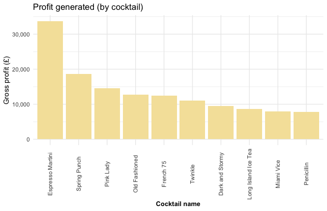
“Espresso Martinis” have generated the most profit fo Suckerpunch - over £30,000 worth! It has outperformed the next best performing drink “Spring Punch” by over a third. These are the drinks that I recommend stay on the next iteration of the menu.
The drinks that yielded the least profit, and which should therefore potentially be removed:
tail(total_gp, 5) %>%
  ggplot(aes(reorder(cocktail, total_gp), y = total_gp)) +
  geom_bar(stat = "identity",  fill = "#f5e2a8") +
  labs(title = "Profit generated (by cocktail)",
       y = "Gross profit (£)",
       x = "Cocktail name") +
  theme_minimal() +
  theme(axis.title.x = element_text(face="bold", size=10),
           axis.text.x  = element_text(angle=90, vjust=0.5)) +
  scale_y_continuous(label = scales::comma)
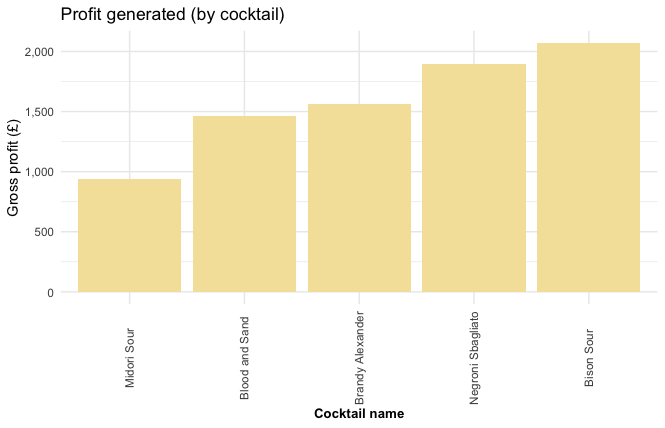
The “Midori Sour” has generated the least profit overall, followed by the charmingly named “Blood and Sand”. These are the drinks I would recommend being replaced on the next iteration of the menu.
Base alcohol popularity
It would be interesting to analyse the popularity of the base alcohol in cocktails over time. To do this, I will have to distill every cocktail down to its (main) base alcohol and plot the data as a time series to see if there have been any changes over time.
Luckily for me, the ingredients data is set out so that the first element is usually the alcohol. This makes extracting the base alcohol for every cocktail much easier.
cocktail <- NULL
alcohol <- NULL

for (each in unique(cocktail_ingredients$cocktail)) {
  x <- cocktail_ingredients %>%
    filter(cocktail == each)
  cocktail <- c(cocktail, unlist(x[1, c(1,4)])[1])
  alcohol <- c(alcohol, unlist(x[1, c(1,4)])[2])
}

cocktail <- data_frame(cocktail)
alcohol <- data_frame(alcohol)

base_alcohol <- bind_cols(cocktail, alcohol)
For the cocktails where the first elements are not the base alcohol, some manual manipulation is required. I’ll also remove “Long Island Ice Tea” since it has so many contributing alcohols.
base_alcohol$alcohol[base_alcohol$alcohol == "Raspberry Puree"] <- "Prosecco"
base_alcohol$alcohol[base_alcohol$alcohol == "MSP Premix"] <- "Prosecco"
base_alcohol$alcohol[base_alcohol$alcohol == "Mezcal"] <- "Tequila"
base_alcohol$alcohol[base_alcohol$alcohol == "Calvados"] <- "Gin"
base_alcohol$alcohol[base_alcohol$alcohol == "Campari"] <- "Prosecco"

base_alcohol <- base_alcohol %>%
  filter(cocktail != "Long Island Ice Tea",
         !alcohol %in% c("Midori"))
Some of the alcohols have different names (“Gin” and “Sloe Gin”) so I’ll do some manipulation to group them together better.
replace_alcohol <- function(a, df) {
  n <- grep(a, df$alcohol)
  df$alcohol <- replace(df$alcohol, n, a)
  return(df$alcohol)
}

base_alcohol$alcohol[base_alcohol$cocktail == "Spring Punch"] <- base_alcohol %>%
  filter(cocktail == "Spring Punch") %>%
  select(alcohol) %>%
  str_replace("Prosecco", "Vodka")


base_alcohol$alcohol <- replace_alcohol("Rum", base_alcohol)
base_alcohol$alcohol <- replace_alcohol("Gin", base_alcohol)

base_alcohol$alcohol[base_alcohol$alcohol == "Zubowka"] <- "Vodka"
base_alcohol$alcohol[base_alcohol$alcohol == "Havana 7yo"] <- "Rum"
I can now merge this table with the sales data and plot the data over a times series.
alcohol_trends <- merge(cocktail_sales, base_alcohol, on = cocktail) %>%
  mutate(date = paste("1", month, year)) %>%
  select(date, alcohol, num_sold) %>%
  group_by(date, alcohol) %>%
  summarise(total_sold = sum(num_sold)) %>%
  filter(date != "2018-08-01") %>%
  arrange(date, alcohol)

alcohol_trends$date <- as.Date(alcohol_trends$date, format = "%d %B %Y")

alcohol_trends %>%
  ggplot(aes(date, total_sold, color = alcohol)) +
  geom_line() +
  labs(title = "Base alcohol consumption in cocktails",
       x = "Date",
       y = "# of cocktails sold",
       color = "Base alcohol") +
  theme_minimal()
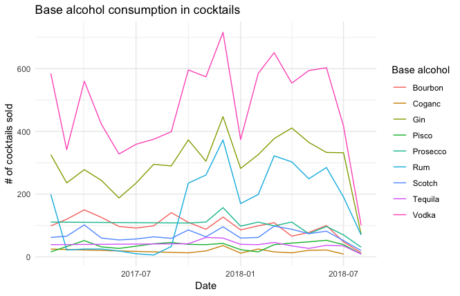
Here we can see that Vodka is by far the most popular base alcohol with little competition. Rum experienced a surge in popularity after Q3 of 2017 (probably due to a menu change around that time). Gin’s popularity has remained constant. It’s worth noting that the decline in sales towards the end of the graph is representative of me taking data halfway through a complete month.
It would also be useful to see these base alcohols as a percentage of total alcohol sales over time.
alcohol_trends %>%
  group_by(date) %>%
  summarise(total_month = sum(total_sold)) %>%
  merge(alcohol_trends, on = date) %>%
  mutate(percent = round((total_sold / total_month)*100, 2)) %>%
  ggplot(aes(date, percent, color = alcohol)) +
  geom_line() +
  labs(title = "Base alcohol consumption in cocktails",
     x = "Date",
     y = "% of total cocktails sold",
     color = "Base alcohol") +
  theme_minimal()
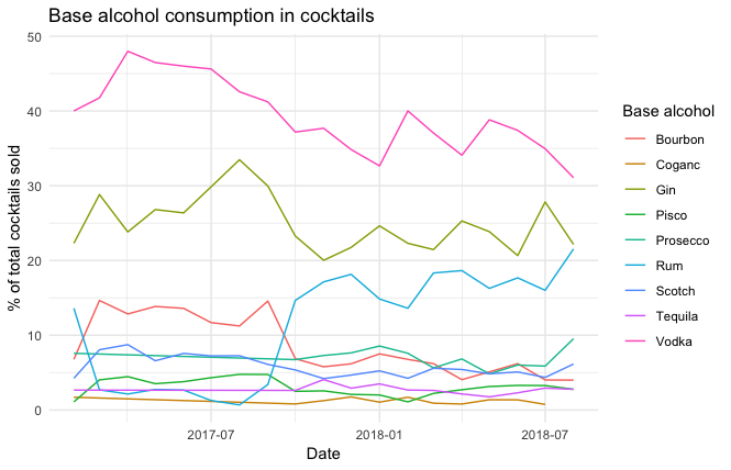
Looking at the data as a percentage of sales in each month gives a much clearer indication of the trends. While we can see that Vodka is still the most popular, we can also see that it’s popularity is waning over time. Gin peaked, dropped and now is at a more-or-less constant second-most popular position. Rum’s increase is still visible, but not more so is Bourbon’s drop in popularity (again, around the time of the menu change).
Cocktail types
The menu is broken into cocktail types, which are loosely based around eras, so it would be interesting to see how these perform against each other.
type <- merge(cocktail_costs, cocktail_sales, on = "cocktail") %>%
   mutate(date = paste("1", month, year)) %>%
  select(date, era, num_sold, total_gp = total) %>%
  group_by(date, era) %>%
  summarise(num_sold = sum(num_sold),
            total = sum(total_gp))


type$date <- as.Date(type$date, format = "%d %B %Y")

type_percent <- type %>%
  group_by(date) %>%
  summarise(total_month = sum(num_sold)) %>%
  merge(type, on = date) %>%
  mutate(percent = round((num_sold / total_month)*100, 2))

type_percent %>%
  ggplot(aes(date, percent, color = era)) +
  geom_line() +
  labs(title = "Cocktail sales by type",
       x = "Date",
       y = "# of cocktails sold",
       color = "Type") +
  theme_minimal()

“Modern Favourites” has consistently been the favourite, although the popularity has steadily decreased over time. “Sucker Punch Favourites” was once the second-most popular type but now finds itself least popular, along with “Prohibition”. The success story here is “Fizzy”, which is now almost-tied for most popular cocktail type. From this, we can determine that “Fizzy” cocktails are good to focus on but some new additions are needed for “Sucker Punch Favourites” and “Modern Favourites”.
type %>%
  select(era, total) %>%
  group_by(era) %>%
  summarise(total = sum(total)) %>%
  ggplot(aes(reorder(era, -total), total)) +
  geom_bar(stat = "identity",  fill = "#f5e2a8") +
  labs(title = "Profit generated (by type)",
     y = "Gross profit (£)",
     x = "Cocktail name") +
  theme_minimal() +
  theme(axis.title.x = element_text(face="bold", size=10),
           axis.text.x  = element_text(angle=90, vjust=0.5)) +
  scale_y_continuous(label = scales::comma)

Unsurprisingly, “Modern Favourites” has generated the most profit since it has been the favoured type for so long. There is opportunity to develop the “Prohibition” and “Cheeky Indulgence” types to maximise profits.
Sharers and shots
In addition to cocktails, the menu also has sharers and shots.
sharers <- c("Skull Puncher", "Miami Vice", "Swizzle", "Spring Punch Skull", "Cosmo skull")
shots <- c("Russian Roulette", "Pick N Mix", "Sangrita City")
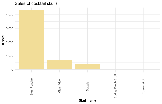
Best selling Skulls
skulls <- cocktail_sales %>%
  filter(cocktail %in% sharers) %>%
  select(cocktail, num_sold, total) %>%
  group_by(cocktail) %>%
  summarise(num_sold = sum(num_sold),
            total = sum(total))

skulls %>%
  ggplot(aes(reorder(cocktail, -num_sold), num_sold)) +
  geom_bar(stat = "identity", fill = "#f5e2a8") +
  labs(title = "Sales of cocktail skulls",
     y = "# sold",
     x = "Skull name") +
  theme_minimal() +
  theme(axis.title.x = element_text(face="bold", size=10),
           axis.text.x  = element_text(angle=90, vjust=0.5)) +
  scale_y_continuous(label = scales::comma)
Most profitable Skulls
skulls %>%
  ggplot(aes(reorder(cocktail, -total), total)) +
  geom_bar(stat = "identity", fill = "#f5e2a8") +
  labs(title = "Revenue (by Skulls)",
     y = "Revenue (£)",
     x = "Skull name") +
  theme_minimal() +
  theme(axis.title.x = element_text(face="bold", size=10),
           axis.text.x  = element_text(angle=90, vjust=0.5)) +
  scale_y_continuous(label = scales::comma)
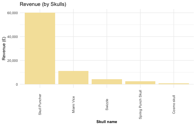
The “Skull Puncher” is the most profitable and best-selling cocktail Skull by far.
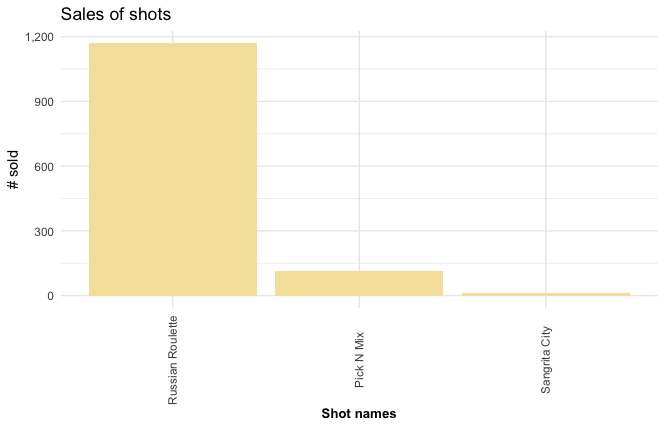
Best selling shots
shots <- cocktail_sales %>%
  filter(cocktail %in% shots) %>%
  select(cocktail, num_sold, total) %>%
  group_by(cocktail) %>%
  summarise(num_sold = sum(num_sold),
            total = sum(total))

shots %>%
  ggplot(aes(reorder(cocktail, -num_sold), num_sold)) +
  geom_bar(stat = "identity", fill = "#f5e2a8") +
  labs(title = "Sales of shots",
     y = "# sold",
     x = "Shot names") +
  theme_minimal() +
  theme(axis.title.x = element_text(face="bold", size=10),
           axis.text.x  = element_text(angle=90, vjust=0.5)) +
  scale_y_continuous(label = scales::comma)
Most profitable shots
shots %>%
  ggplot(aes(reorder(cocktail, -total), total)) +
  geom_bar(stat = "identity", fill = "#f5e2a8") +
  labs(title = "Revenue (by shots)",
     y = "Revenue (£)",
     x = "Shot names") +
  theme_minimal() +
  theme(axis.title.x = element_text(face="bold", size=10),
           axis.text.x  = element_text(angle=90, vjust=0.5)) +
  scale_y_continuous(label = scales::comma)
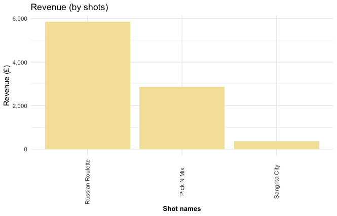
The “Russian Roulette” shots are the best performing in both sales and profit.
Off-menu drinks
It will also be interesting to see the best-selling off-menu orders, to see if there are any additions it would be worth adding.
off_menu <- anti_join(cocktail_sales, cocktail_costs, by = "cocktail") %>%
  select(cocktail, num_sold, total) %>%
  group_by(cocktail) %>%
  summarise(num_sold = sum(num_sold),
           total = sum(total)) %>%
  arrange(desc(num_sold))

remove <- c("Open Drink 2", "Open drink 3", "Open drink 1", "Open drink 4")

off_menu <- off_menu %>%
  filter(!cocktail %in% remove) %>%
  anti_join(skulls, on = cocktail) %>%
  anti_join(shots, on = cocktail)
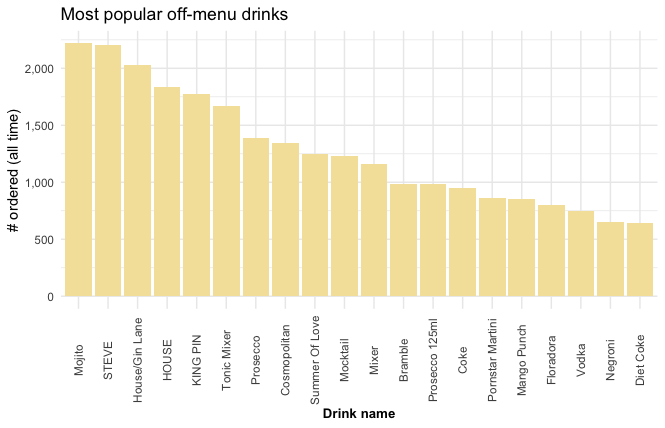
Most popular off-menu drinks
off_menu %>%
  head(20) %>%
  ggplot(aes(reorder(cocktail, -num_sold), num_sold)) +
  geom_bar(stat = "identity",  fill = "#f5e2a8") +
  labs(title = "Most popular off-menu drinks",
     y = "# ordered (all time)",
     x = "Drink name") +
  theme_minimal() +
  theme(axis.title.x = element_text(face="bold", size=10),
           axis.text.x  = element_text(angle=90, vjust=0.5)) +
  scale_y_continuous(label = scales::comma)
Off-menu drinks that have yielded the most revenue
off_menu %>%
  head(20) %>%
  ggplot(aes(reorder(cocktail, -total), total)) +
  geom_bar(stat = "identity",  fill = "#f5e2a8") +
  labs(title = "Off-menu drinks that have yielded the most revenue",
     y = "Revenue (£)",
     x = "Drink name") +
  theme_minimal() +
  theme(axis.title.x = element_text(face="bold", size=10),
           axis.text.x  = element_text(angle=90, vjust=0.5)) +
  scale_y_continuous(label = scales::comma)
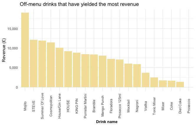
While the “Mojito” and the “STEVE” (a beer) have sold almost the same amount, the “Mojito” has yielded a lot more revenue. The “Summer Of Love” and the “Cosmopolitan” would also be good additions to the menu.
Conclusion
This is the final blog post pertaining to the “Putting the R in Bar” project. I presented my findings at the EARL conference on 12th September 2018. In future blog posts, I will show how I put all of these findings into a shiny app with an interface easy enough for a non-technical user.