Predicting profit generated by movies
Python
In my last post, I tested several models that predicted movie ratings. This time, I’ll try and predict the gross profit a movie might generate based on the same features. The aim is to create a Flask app that will allow a user to see the predicted rating and gross profit for a movie they create based on certain feature choices (ie. cast, director, genre).
Since all the data cleaning was done in my last blog post, I can move straight into the exploratory data analysis.
Set up and import data
import pandas as pd
import numpy as np

from matplotlib import pyplot as plt
import seaborn as sns
import pickle

from sklearn import linear_model as lm, metrics, tree, ensemble, svm
from sklearn.model_selection import train_test_split, KFold, cross_val_score, GridSearchCV
from sklearn.preprocessing import StandardScaler

%matplotlib inline

pd.options.mode.chained_assignment = None
pd.set_option('display.max_columns', 500)
pd.set_option('display.max_rows', 5000)

np.random.seed(42)
sns.set(rc={
    'figure.figsize': (12, 8),
    'font.size': 14
})

# Set palette
sns.set_palette("husl")
movies = pd.read_csv("/Users/jasminepengelly/Desktop/projects/predicting_movie/movies_wo_dir.csv")
movies.drop("Unnamed: 0", axis=1, inplace=True)
movies["gross_profit"] = movies["revenue"] - movies["budget"]
movies.head()
| title | id | budget | revenue | runtime | vote_average | vote_count | belongs_to_collection | Action | Adventure | Animation | Aniplex | BROSTA TV | Carousel Productions | Comedy | Crime | Documentary | Drama | Family | Fantasy | Foreign | GoHands | History | Horror | Mardock Scramble Production Committee | Music | Mystery | Odyssey Media | Pulser Productions | Rogue State | Romance | Science Fiction | Sentai Filmworks | TV Movie | Telescene Film Group Productions | The Cartel | Thriller | Vision View Entertainment | War | Western | lead | supporting | dir_count | gross_profit | |
|---|---|---|---|---|---|---|---|---|---|---|---|---|---|---|---|---|---|---|---|---|---|---|---|---|---|---|---|---|---|---|---|---|---|---|---|---|---|---|---|---|---|---|---|---|
| 0 | Toy Story | 862 | 30000000.0 | 373554033.0 | 81.0 | 7.7 | 5415.0 | 1 | 0.0 | 0.0 | 1.0 | 0.0 | 0.0 | 0.0 | 1.0 | 0.0 | 0.0 | 0.0 | 1.0 | 0.0 | 0.0 | 0.0 | 0.0 | 0.0 | 0.0 | 0.0 | 0.0 | 0.0 | 0.0 | 0.0 | 0.0 | 0.0 | 0.0 | 0.0 | 0.0 | 0.0 | 0.0 | 0.0 | 0.0 | 0.0 | Tom Hanks | Tim Allen | 5 | 343554033.0 |
| 1 | Jumanji | 8844 | 65000000.0 | 262797249.0 | 104.0 | 6.9 | 2413.0 | 0 | 0.0 | 1.0 | 0.0 | 0.0 | 0.0 | 0.0 | 0.0 | 0.0 | 0.0 | 0.0 | 1.0 | 1.0 | 0.0 | 0.0 | 0.0 | 0.0 | 0.0 | 0.0 | 0.0 | 0.0 | 0.0 | 0.0 | 0.0 | 0.0 | 0.0 | 0.0 | 0.0 | 0.0 | 0.0 | 0.0 | 0.0 | 0.0 | Robin Williams | Jonathan Hyde | 7 | 197797249.0 |
| 2 | Heat | 949 | 60000000.0 | 187436818.0 | 170.0 | 7.7 | 1886.0 | 0 | 1.0 | 0.0 | 0.0 | 0.0 | 0.0 | 0.0 | 0.0 | 1.0 | 0.0 | 1.0 | 0.0 | 0.0 | 0.0 | 0.0 | 0.0 | 0.0 | 0.0 | 0.0 | 0.0 | 0.0 | 0.0 | 0.0 | 0.0 | 0.0 | 0.0 | 0.0 | 0.0 | 0.0 | 1.0 | 0.0 | 0.0 | 0.0 | Al Pacino | Robert De Niro | 10 | 127436818.0 |
| 3 | Sudden Death | 9091 | 35000000.0 | 64350171.0 | 106.0 | 5.5 | 174.0 | 0 | 1.0 | 1.0 | 0.0 | 0.0 | 0.0 | 0.0 | 0.0 | 0.0 | 0.0 | 0.0 | 0.0 | 0.0 | 0.0 | 0.0 | 0.0 | 0.0 | 0.0 | 0.0 | 0.0 | 0.0 | 0.0 | 0.0 | 0.0 | 0.0 | 0.0 | 0.0 | 0.0 | 0.0 | 1.0 | 0.0 | 0.0 | 0.0 | Jean-Claude Van Damme | Powers Boothe | 10 | 29350171.0 |
| 4 | GoldenEye | 710 | 58000000.0 | 352194034.0 | 130.0 | 6.6 | 1194.0 | 1 | 1.0 | 1.0 | 0.0 | 0.0 | 0.0 | 0.0 | 0.0 | 0.0 | 0.0 | 0.0 | 0.0 | 0.0 | 0.0 | 0.0 | 0.0 | 0.0 | 0.0 | 0.0 | 0.0 | 0.0 | 0.0 | 0.0 | 0.0 | 0.0 | 0.0 | 0.0 | 0.0 | 0.0 | 1.0 | 0.0 | 0.0 | 0.0 | Pierce Brosnan | Sean Bean | 8 | 294194034.0 |
Exploratory data analysis
From my previous analysis, I know there is a relatively high correlation between budget, revenue and vote_count. This time around I’ll focus on the relationships between revenue and the other variables.
First, I’ll define the variables that I’m using.
X = ['budget', 'runtime', 'vote_count', 'belongs_to_collection', 'Action', 'Adventure',
              'Animation', 'Aniplex', 'BROSTA TV', 'Carousel Productions', 'Comedy', 'Crime', 'Documentary', 'Drama',
              'Family', 'Fantasy', 'Foreign', 'GoHands', 'History', 'Horror', 'Mardock Scramble Production Committee',
              'Music', 'Mystery', 'Odyssey Media', 'Pulser Productions', 'Rogue State', 'Romance', 'Science Fiction',
              'Sentai Filmworks', 'TV Movie', 'Telescene Film Group Productions', 'The Cartel', 'Thriller',
              'Vision View Entertainment', 'War', 'Western', 'lead', 'supporting', 'vote_average']

y = 'gross_profit'
sns.heatmap(movies.drop(['title', 'id', 'dir_count'], axis=1).corr(), vmin=-1, vmax=1, center=0, cmap=sns.diverging_palette(10, 220, sep=80, n=7))
<matplotlib.axes._subplots.AxesSubplot at 0x1a1aabd240>
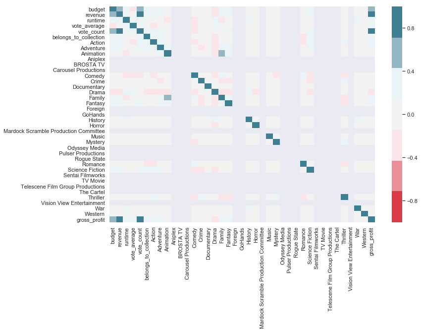
My response variable, gross_profit, is highly correlated with budget, revenue and vote_ count. budget and revenue make sense, since the three are directly related, but vote_ count is less intuitive - perhaps more votes are to be expected on popular films, and films with a high budget or that make large revenue get more votes.
Within my features, I already identified the correlation between Family and Animation, and vote_count and budget, are not significant enough to worry about. This bodes well for my models - there will be no multicollinearity and there is no need for PCA here.
Highest revenue films
high_rev = movies[['title', 'revenue']].sort_values(by = 'revenue', ascending = False).head(10)
high_rev['revenue'] = high_rev['revenue'].map('${:,.2f}'.format)
high_rev
| title | revenue | |
|---|---|---|
| 1439 | Avatar | $2,787,965,087.00 |
| 1766 | Star Wars: The Force Awakens | $2,068,223,624.00 |
| 328 | Titanic | $1,845,034,188.00 |
| 1778 | Furious 7 | $1,506,249,360.00 |
| 1540 | Harry Potter and the Deathly Hallows: Part 2 | $1,342,000,000.00 |
| 1875 | Beauty and the Beast | $1,262,886,337.00 |
| 1881 | The Fate of the Furious | $1,238,764,765.00 |
| 1535 | Transformers: Dark of the Moon | $1,123,746,996.00 |
| 994 | The Lord of the Rings: The Return of the King | $1,118,888,979.00 |
| 1614 | Skyfall | $1,108,561,013.00 |
Highest grossing films
high_gp = movies[['title', "gross_profit"]].sort_values(by = "gross_profit", ascending = False).head(10)
high_gp["gross_profit"] = high_gp["gross_profit"].map('${:,.2f}'.format)
high_gp
| title | gross_profit | |
|---|---|---|
| 1439 | Avatar | $2,550,965,087.00 |
| 1766 | Star Wars: The Force Awakens | $1,823,223,624.00 |
| 328 | Titanic | $1,645,034,188.00 |
| 1778 | Furious 7 | $1,316,249,360.00 |
| 1540 | Harry Potter and the Deathly Hallows: Part 2 | $1,217,000,000.00 |
| 1875 | Beauty and the Beast | $1,102,886,337.00 |
| 994 | The Lord of the Rings: The Return of the King | $1,024,888,979.00 |
| 1881 | The Fate of the Furious | $988,764,765.00 |
| 1535 | Transformers: Dark of the Moon | $928,746,996.00 |
| 1614 | Skyfall | $908,561,013.00 |
Lowest revenue films
low_rev = movies[['title', 'revenue']].sort_values(by = 'revenue', ascending = True).head(10)
low_rev['revenue'] = low_rev['revenue'].map('${:,.2f}'.format)
low_rev
| title | revenue | |
|---|---|---|
| 576 | Angela's Ashes | $13.00 |
| 1271 | Death at a Funeral | $46.00 |
| 628 | The Idiots | $7,235.00 |
| 1604 | 5 Days of War | $17,479.00 |
| 590 | City Lights | $19,181.00 |
| 1464 | Valhalla Rising | $30,638.00 |
| 480 | Following | $48,482.00 |
| 1678 | The Canyons | $56,825.00 |
| 1628 | Byzantium | $89,237.00 |
| 1796 | Manglehorn | $143,101.00 |
Biggest loss
high_gp = movies[['title', "gross_profit"]].sort_values(by = "gross_profit", ascending = True).head(10)
high_gp["gross_profit"] = high_gp["gross_profit"].map('${:,.2f}'.format)
high_gp
| title | gross_profit | |
|---|---|---|
| 1673 | The Lone Ranger | $-165,710,090.00 |
| 1011 | The Alamo | $-119,180,039.00 |
| 1884 | Valerian and the City of a Thousand Planets | $-107,447,384.00 |
| 513 | The 13th Warrior | $-98,301,101.00 |
| 7 | Cutthroat Island | $-87,982,678.00 |
| 1365 | Australia | $-80,445,998.00 |
| 578 | Supernova | $-75,171,919.00 |
| 1080 | A Sound of Thunder | $-74,010,360.00 |
| 1128 | The Great Raid | $-69,833,498.00 |
| 1674 | R.I.P.D. | $-68,351,500.00 |
Import directors and get dummy variables
directors = pd.read_csv("/Users/jasminepengelly/Desktop/projects/predicting_movie/director_dummies.csv")
directors.drop("Unnamed: 0", axis=1, inplace=True)
final = pd.merge(directors, movies, left_on = 'index', right_on = 'id')
final.drop(["id", "index", "title", "dir_count"], axis=1, inplace=True)
dummies = pd.get_dummies(final, columns=['lead', 'supporting'], drop_first=True)
Pre-processing
Since the final product of this modelling is to produce a Flask app that allows someone to input factors about a film before it’s produced to get the rating and the gross profit generated, some features will have to be dropped. For example, a user would not know the vote_count before the film is created. Some of the features I am removing are the most correlated with the response variable so I will be losing some of the predictive power.
I’ll begin by defining my train-test split. Then, as with my previous blog post, I’ll standardise the remaining predictive variables since it’s good practice for working with linear regression models.
X = dummies.drop(["revenue", "vote_count", "gross_profit", "vote_average"], axis=1)
y = dummies["gross_profit"]
scaler = StandardScaler()
X_train, X_test, y_train, y_test = train_test_split(X, y, test_size=0.3, random_state=42)
X_train = pd.DataFrame(scaler.fit_transform(X_train), columns=X.columns)
X_test = pd.DataFrame(scaler.transform(X_test), columns=X.columns)
print("Length of training sets:",len(X_train), len(X_test))
print("Length of testing sets:",len(y_train), len(y_test))
Length of training sets: 1320 567
Length of testing sets: 1320 567
Modelling
Baseline score
I need a baseline score with which to compare the scores for all my models moving forward. This score will represent the score one would get if they were just to predict the mean value for y. If my model outperforms this score, I know it is doing well.
y_pred_mean = [y_train.mean()] * len(y_test)

print("Dumb model RMSE: ",'${:,.2f}'.format(np.sqrt(metrics.mean_squared_error(y_test, y_pred_mean))))
Dumb model RMSE: $226,516,599.51
$226 million will be the benchmark RMSE for my model’s success. It’s still a very wide margin to be out by, so I’m hoping I can beat this.
Function to generate model scores
Since I’ll be trying out many different models, I’ll build a function that returns all the information for efficiency. I’ll create one function for simple models and another for models utilising regularisation.
If this were a function I was using regularly, I would put it in a script and import it. However, I wanted it explicitly stated here for you to see.
# Function to return simple model metrics
def get_model_metrics(X_train, y_train, X_test, y_test, model, parametric=True):
    """This function takes the train-test splits as arguments, as well as the algorithm
    being used, and returns the training score, the test score (both RMSE), the
    cross-validated scores and the mean cross-validated score. It also returns the appropriate
    feature importances depending on whether the optional argument 'parametric' is equal to
    True or False."""

    model.fit(X_train, y_train)
    train_pred = np.around(model.predict(X_train),1)
    test_pred = np.around(model.predict(X_test),1)

    print('Training RMSE:', '${:,.2f}'.format(np.sqrt(metrics.mean_squared_error(y_train, train_pred))))
    print('Testing RMSE:', '${:,.2f}'.format(np.sqrt(metrics.mean_squared_error(y_test, test_pred))))
    cv_scores = -cross_val_score(model, X_train, y_train, cv=5, scoring='neg_mean_squared_error')
    print('Cross-validated RMSEs:', np.sqrt(cv_scores))
    print('Mean cross-validated RMSE:', '${:,.2f}'.format(np.sqrt(np.mean(cv_scores))))

    if parametric == True:
        print(pd.DataFrame(list(zip(X_train.columns, model.coef_, abs(model.coef_))),
                 columns=['Feature', 'Coef', 'Abs Coef']).sort_values('Abs Coef', ascending=False).head(10))
    else:
        print(pd.DataFrame(list(zip(X_train.columns, model.feature_importances_)),
                 columns=['Feature', 'Importance']).sort_values('Importance', ascending=False).head(10))

    return model
# Function to return regularised model metrics
def regularised_model_metrics(X_train, y_train, X_test, y_test, model, grid_params, parametric=True):
    """This function takes the train-test splits as arguments, as well as the algorithm being
    used and the parameters, and returns the best cross-validated training score, the test
    score, the best performing model and it's parameters, and the feature importances."""

    gridsearch = GridSearchCV(model,
                              grid_params,
                              n_jobs=-1, cv=5, verbose=1, error_score='neg_mean_squared_error')

    gridsearch.fit(X_train, y_train)
    print('Best parameters:', gridsearch.best_params_)
    print('Cross-validated score on test data:', '${:,.2f}'.format(abs(gridsearch.best_score_)))
    best_model = gridsearch.best_estimator_
    print('Testing RMSE:', '${:,.2f}'.format(np.sqrt(metrics.mean_squared_error(y_test, best_model.predict(X_test)))))

    if parametric == True:
        print(pd.DataFrame(list(zip(X_train.columns, best_model.coef_, abs(best_model.coef_))),
                 columns=['Feature', 'Coef', 'Abs Coef']).sort_values('Abs Coef', ascending=False).head(10))
    else:
        print(pd.DataFrame(list(zip(X_train.columns, best_model.feature_importances_)),
                 columns=['Feature', 'Importance']).sort_values('Importance', ascending=False).head(10))

    return best_model
Linear regression
Simple
lr = get_model_metrics(X_train, y_train, X_test, y_test, lm.LinearRegression())
lr
Training RMSE: $43,093,674.65
Testing RMSE: $6,850,145,181,265,346,691,072.00
Cross-validated RMSEs: [4.17892339e+21 9.90531764e+21 1.53491007e+22 1.13727100e+22
 5.58558345e+21]
Mean cross-validated RMSE: $10,116,431,047,916,374,720,512.00
                                    Feature          Coef      Abs Coef
1088              supporting_Bijou Phillips  1.347614e+21  1.347614e+21
276        Telescene Film Group Productions -1.259300e+21  1.259300e+21
266   Mardock Scramble Production Committee  1.202241e+21  1.202241e+21
665                         lead_Judi Dench -1.150649e+21  1.150649e+21
1951                  supporting_Seth Green -1.078695e+21  1.078695e+21
584                        lead_James Woods -1.075888e+21  1.075888e+21
428                   lead_Cuba Gooding Jr.  1.031542e+21  1.031542e+21
25                              Bill Condon  1.029315e+21  1.029315e+21
1212                 supporting_Dan Stevens -1.012743e+21  1.012743e+21
1011            supporting_Adrienne Barbeau -9.823532e+20  9.823532e+20


LinearRegression(copy_X=True, fit_intercept=True, n_jobs=1, normalize=False)
Both my scores are terrible here, and the vast difference between the scores show the level of overfitting. Time for some regularisation.
Regularised - Ridge
ridge = lm.Ridge()

ridge_params = {'alpha': np.linspace(600, 800, 5),
               'fit_intercept': [True, False],
               'solver': ['auto', 'svd', 'cholesky', 'lsqr', 'sparse_cg', 'sag', 'saga']}

ridge_model = regularised_model_metrics(X_train, y_train, X_test, y_test, ridge, ridge_params)
Fitting 5 folds for each of 70 candidates, totalling 350 fits


[Parallel(n_jobs=-1)]: Done  42 tasks      | elapsed:    9.3s
[Parallel(n_jobs=-1)]: Done 192 tasks      | elapsed:   35.6s
[Parallel(n_jobs=-1)]: Done 350 out of 350 | elapsed:  1.1min finished


Best parameters: {'alpha': 700.0, 'fit_intercept': True, 'solver': 'saga'}
Cross-validated score on test data: $0.36
Testing RMSE: $185,680,100.81
                       Feature          Coef      Abs Coef
249      belongs_to_collection  2.131550e+07  2.131550e+07
247                     budget  2.086358e+07  2.086358e+07
82                George Lucas  1.426045e+07  1.426045e+07
248                    runtime  1.330278e+07  1.330278e+07
437      lead_Daniel Radcliffe  1.128897e+07  1.128897e+07
1918   supporting_Rupert Grint  1.100804e+07  1.100804e+07
1976  supporting_Stanley Tucci  9.935829e+06  9.935829e+06
1395   supporting_Ian McKellen  9.889183e+06  9.889183e+06
251                  Adventure  9.849955e+06  9.849955e+06
491           lead_Emma Watson  9.219124e+06  9.219124e+06
This test score is already better than the baseline, so I know we are moving in the right direction. With the most predictive features removed, it’s interesting to see that ‘belongs_to_collection’ seems to be more influencial than budget.
Regularised - Lasso
lasso = lm.Lasso(tol=5)

lasso_params = {'alpha': np.logspace(10, 100, 5),
               'fit_intercept': [True, False]}

lasso_model = regularised_model_metrics(X_train, y_train, X_test, y_test, lasso, lasso_params)
Fitting 5 folds for each of 10 candidates, totalling 50 fits


[Parallel(n_jobs=-1)]: Done  42 tasks      | elapsed:    2.6s


Best parameters: {'alpha': 10000000000.0, 'fit_intercept': True}
Cross-validated score on test data: $0.02
Testing RMSE: $226,516,599.51
                        Feature  Coef  Abs Coef
0                 Aaron Seltzer  -0.0       0.0
1402   supporting_Irene Miracle   0.0       0.0
1400  supporting_Ingrid Bergman   0.0       0.0
1399    supporting_Ichirō Nagai  -0.0       0.0
1398        supporting_Ice Cube   0.0       0.0
1397     supporting_Iben Hjejle  -0.0       0.0
1396     supporting_Ian McShane   0.0       0.0
1395    supporting_Ian McKellen   0.0       0.0
1394   supporting_Ian McDiarmid   0.0       0.0
1393        supporting_Ian Holm   0.0       0.0


[Parallel(n_jobs=-1)]: Done  50 out of  50 | elapsed:    3.0s finished
After a lot of tuning and increasing the alpha, lasso still didn’t perform as well as ridge. The coefficients also make less intuitive sense.
Regularised - ElasticNet
elastic = lm.ElasticNet()

elastic_params = {'alpha': np.linspace(1, 10, 10),
                 'l1_ratio': np.linspace(0.05, 0.95, 10),
                 'fit_intercept': [True, False]}

elastic_model = regularised_model_metrics(X_train, y_train, X_test, y_test, elastic,
                                          elastic_params)
Fitting 5 folds for each of 200 candidates, totalling 1000 fits


[Parallel(n_jobs=-1)]: Done  42 tasks      | elapsed:    4.7s
[Parallel(n_jobs=-1)]: Done 192 tasks      | elapsed:   19.4s
[Parallel(n_jobs=-1)]: Done 442 tasks      | elapsed:   34.3s
[Parallel(n_jobs=-1)]: Done 792 tasks      | elapsed:   53.1s


Best parameters: {'alpha': 2.0, 'fit_intercept': True, 'l1_ratio': 0.65}
Cross-validated score on test data: $0.36
Testing RMSE: $186,283,469.11
                       Feature          Coef      Abs Coef
247                     budget  1.991908e+07  1.991908e+07
249      belongs_to_collection  1.967256e+07  1.967256e+07
82                George Lucas  1.289770e+07  1.289770e+07
248                    runtime  1.227358e+07  1.227358e+07
437      lead_Daniel Radcliffe  1.076488e+07  1.076488e+07
1918   supporting_Rupert Grint  1.046807e+07  1.046807e+07
251                  Adventure  9.455739e+06  9.455739e+06
1395   supporting_Ian McKellen  9.207659e+06  9.207659e+06
1976  supporting_Stanley Tucci  9.097251e+06  9.097251e+06
1212    supporting_Dan Stevens  8.682729e+06  8.682729e+06


[Parallel(n_jobs=-1)]: Done 1000 out of 1000 | elapsed:  1.1min finished
This gives me very similar results to the ridge linear regression, but still doesn’t perform as well. So far, the ridge linear regression is the best performing.
Tree models
Simple decision tree
dt = get_model_metrics(X_train, y_train, X_test, y_test, tree.DecisionTreeRegressor(),
                       parametric=False)
dt
Training RMSE: $0.00
Testing RMSE: $189,435,992.34
Cross-validated RMSEs: [1.62986560e+08 1.50676461e+08 1.16390236e+08 1.28971798e+08
 1.60756615e+08]
Mean cross-validated RMSE: $145,114,517.27
                       Feature  Importance
247                     budget    0.330288
249      belongs_to_collection    0.124512
248                    runtime    0.096301
491           lead_Emma Watson    0.026973
742           lead_Mark Hamill    0.013669
37                Bryan Singer    0.012596
799            lead_Neel Sethi    0.012294
42           Christopher Nolan    0.011744
278                   Thriller    0.011406
2028  supporting_Toni Collette    0.010859


DecisionTreeRegressor(criterion='mse', max_depth=None, max_features=None,
           max_leaf_nodes=None, min_impurity_decrease=0.0,
           min_impurity_split=None, min_samples_leaf=1,
           min_samples_split=2, min_weight_fraction_leaf=0.0,
           presort=False, random_state=None, splitter='best')
Simple decision trees tend to overfit, so I am not surprised by the train and test scores being what they are. However, I am surprised that the cross-validated score is quite good.
Random forest
rf = get_model_metrics(X_train, y_train, X_test, y_test, ensemble.RandomForestRegressor(),
                       parametric=False)
rf
Training RMSE: $51,290,496.58
Testing RMSE: $171,985,754.15
Cross-validated RMSEs: [1.30170546e+08 1.29842827e+08 9.17430304e+07 1.19111377e+08
 1.27713356e+08]
Mean cross-validated RMSE: $120,597,293.25
                       Feature  Importance
247                     budget    0.324819
249      belongs_to_collection    0.119175
248                    runtime    0.073327
25                 Bill Condon    0.012158
226           Steven Spielberg    0.012097
742           lead_Mark Hamill    0.011958
2028  supporting_Toni Collette    0.011653
1395   supporting_Ian McKellen    0.010731
799            lead_Neel Sethi    0.010293
251                  Adventure    0.009515


RandomForestRegressor(bootstrap=True, criterion='mse', max_depth=None,
           max_features='auto', max_leaf_nodes=None,
           min_impurity_decrease=0.0, min_impurity_split=None,
           min_samples_leaf=1, min_samples_split=2,
           min_weight_fraction_leaf=0.0, n_estimators=10, n_jobs=1,
           oob_score=False, random_state=None, verbose=0, warm_start=False)
The best performing model so far, with feature importances that make intuitive sense.
Regularised Random forest
rrf = ensemble.RandomForestRegressor()

rrf_params = {'bootstrap': [True, False],
             'max_depth': np.linspace(5, 50, 5),
             'min_samples_split': np.linspace(0.1, 1, 5),
             'n_estimators': [10, 15, 20]}

rrf_model = regularised_model_metrics(X_train, y_train, X_test, y_test, rrf, rrf_params,
                                     parametric=False)
Fitting 5 folds for each of 150 candidates, totalling 750 fits


[Parallel(n_jobs=-1)]: Done  42 tasks      | elapsed:    3.4s
[Parallel(n_jobs=-1)]: Done 192 tasks      | elapsed:   16.4s
[Parallel(n_jobs=-1)]: Done 442 tasks      | elapsed:   42.7s
[Parallel(n_jobs=-1)]: Done 750 out of 750 | elapsed:  1.7min finished


Best parameters: {'bootstrap': False, 'max_depth': 5.0, 'min_samples_split': 0.1, 'n_estimators': 10}
Cross-validated score on test data: $0.35
Testing RMSE: $188,255,673.77
                       Feature  Importance
247                     budget    0.628325
249      belongs_to_collection    0.270686
2028  supporting_Toni Collette    0.023607
248                    runtime    0.015528
742           lead_Mark Hamill    0.014858
1371  supporting_Harrison Ford    0.014858
226           Steven Spielberg    0.013352
678      lead_Kathryn Beaumont    0.009393
2046   supporting_Verna Felton    0.009393
1395   supporting_Ian McKellen    0.000000
A good test score, but not quite as good as the random forest with the default parameters.
Bagged decision trees
bagdt = ensemble.BaggingRegressor()
bagdt.fit(X_train, y_train)

print('Training RMSE:', '${:,.2f}'.format(np.sqrt(metrics.mean_squared_error(y_train, bagdt.predict(X_train)))))
print('Testing RMSE:', '${:,.2f}'.format(np.sqrt(metrics.mean_squared_error(y_test, bagdt.predict(X_test)))))
cv_scores = -cross_val_score(bagdt, X_train, y_train, cv=5, scoring='neg_mean_squared_error')
print('Cross-validated RMSEs:', cv_scores)
print('Mean cross-validated RMSE:', '${:,.2f}'.format(np.mean(cv_scores)))
Training RMSE: $47,551,713.19
Testing RMSE: $167,557,918.72
Cross-validated RMSEs: [1.61524815e+16 1.63382135e+16 8.80421032e+15 1.40081532e+16
 1.70218650e+16]
Mean cross-validated RMSE: $14,464,984,700,217,268.00
I am disappointed at the mean cross-validated score here - this model won’t generalise well.
Support Vector Machine
LinearSVR
lin = svm.LinearSVR()

lin_params = {
    'C': np.logspace(-3, 2, 5),
    'loss': ['epsilon_insensitive','squared_epsilon_insensitive'],
    'fit_intercept': [True,False],
    'max_iter': [1000]
}

lin_model = regularised_model_metrics(X_train, y_train, X_test, y_test, lin, lin_params)
Fitting 5 folds for each of 20 candidates, totalling 100 fits


[Parallel(n_jobs=-1)]: Done  42 tasks      | elapsed:    4.6s
[Parallel(n_jobs=-1)]: Done 100 out of 100 | elapsed:   53.0s finished


Best parameters: {'C': 0.001, 'fit_intercept': True, 'loss': 'squared_epsilon_insensitive', 'max_iter': 1000}
Cross-validated score on test data: $0.07
Testing RMSE: $188,783,310.28
                       Feature          Coef      Abs Coef
249      belongs_to_collection  2.347037e+07  2.347037e+07
247                     budget  2.172464e+07  2.172464e+07
82                George Lucas  1.620963e+07  1.620963e+07
248                    runtime  1.470311e+07  1.470311e+07
437      lead_Daniel Radcliffe  1.180886e+07  1.180886e+07
1918   supporting_Rupert Grint  1.154390e+07  1.154390e+07
1976  supporting_Stanley Tucci  1.089841e+07  1.089841e+07
1395   supporting_Ian McKellen  1.066900e+07  1.066900e+07
251                  Adventure  1.028434e+07  1.028434e+07
2028  supporting_Toni Collette  1.008356e+07  1.008356e+07
Although the test score is below baseline, the test score isn’t as good as the random forest.
RBF
rbf = svm.SVR(kernel='rbf')

rbf_params = {
    'C': np.logspace(-3, 2, 5),
    'gamma': np.logspace(-3, 2, 5),
    'kernel': ['rbf']}

rbf = GridSearchCV(rbf, rbf_params, n_jobs=-1, cv=5, verbose=1, error_score='neg_mean_squared_error')
rbf.fit(X_train, y_train)
print('Best parameters:', rbf.best_params_)
print('Training RMSE:', '${:,.2f}'.format(abs(rbf.best_score_)))
print('Testing RMSE:', '${:,.2f}'.format(np.sqrt(metrics.mean_squared_error(y_test, rbf.best_estimator_.predict(X_test)))))
Fitting 5 folds for each of 25 candidates, totalling 125 fits


[Parallel(n_jobs=-1)]: Done  42 tasks      | elapsed:  1.5min
[Parallel(n_jobs=-1)]: Done 125 out of 125 | elapsed:  4.1min finished


Best parameters: {'C': 100.0, 'gamma': 0.001, 'kernel': 'rbf'}
Training RMSE: $0.14
Testing RMSE: $240,436,736.27
This has performed worse than the LinearSVR, so I won’t be using this.
Poly
poly = svm.SVR(kernel='poly')

poly_params = {
    'C': np.logspace(-3, 2, 3),
    'gamma': np.logspace(-5, 2, 3),
    'degree': [2]}

poly = GridSearchCV(poly, poly_params, n_jobs=-1, cv=5, verbose=1, error_score='neg_mean_squared_error')
poly.fit(X_train, y_train)
print('Best parameters:', poly.best_params_)
print('Training RMSE:', '${:,.2f}'.format(abs(poly.best_score_)))
print('Testing RMSE:', '${:,.2f}'.format(np.sqrt(metrics.mean_squared_error(y_test, poly.best_estimator_.predict(X_test)))))
Fitting 5 folds for each of 9 candidates, totalling 45 fits


[Parallel(n_jobs=-1)]: Done  45 out of  45 | elapsed:  1.5min finished


Best parameters: {'C': 0.31622776601683794, 'degree': 2, 'gamma': 100.0}
Training RMSE: $0.14
Testing RMSE: $202,171,501.80
I did play with including 3 as a degree hyperparameter, but the gridsearch took ages to run and the results didn’t improve much.
Conclusion
The best performing model is the random forest. I will pickle it, as well as exporting the scaled features as csv, and use them in my Flask app.
X_scaled = pd.concat([X_train, X_test])
y_concat = pd.concat([y_train, y_test])
X_scaled.to_csv("X_profit.csv")
rf.fit(X_scaled, y_concat)
cv_scores = -cross_val_score(rf, X_scaled, y_concat, cv=5, scoring='neg_mean_squared_error')
print('Cross-validated RMSEs:', np.sqrt(cv_scores))
print('Mean cross-validated RMSE:', '${:,.2f}'.format(np.mean(np.sqrt(cv_scores))))
Cross-validated RMSEs: [1.25429824e+08 9.88043543e+07 1.11233629e+08 1.53454944e+08
 1.52458683e+08]
Mean cross-validated RMSE: $128,276,286.95
with open('model_profit.pkl', 'wb') as f:
    pickle.dump(rf, f)