Predicting IMDB ratings for movies
Python
I consider myself an enthusiastic, if not particularly knowledgable, cinephile. When debating between multiple movies to watch, my partner and I always do the “IMDB test” - the movie we choose is the one with the highest average rating on IMDB (I plan to create a movie recommender system to replace this method at some point, but that’s another blog post). I would like to see how easy it could be to predict the average rating for a movie, and what predictors have the most effect.
The dataset I used is the popular Movies dataset found on Kaggle. The aim is to try different models and find the one with the lowest root mean squared error (RMSE).
Once I have identified the best performing model, I will create a Flask app to allow users to create their own movies using the given feature options (cast, crew etc) and predict the rating and the revenue it would generate. It would also be worth hooking this up to the OMBd API to get the most up-to-date movie information.
import pandas as pd
import numpy as np
import pickle

from matplotlib import pyplot as plt
from matplotlib_venn import venn2
import seaborn as sns

from sklearn import linear_model as lm, metrics, tree, ensemble, model_selection as ms, feature_selection, svm
from sklearn.preprocessing import StandardScaler
from sklearn.model_selection import GridSearchCV

%matplotlib inline

pd.options.mode.chained_assignment = None

np.random.seed(42)

import warnings
warnings.filterwarnings("ignore")
sns.set(rc={
    'figure.figsize': (12, 8),
    'font.size': 14
})

# Set palette
sns.set_palette("husl")
pd.set_option('display.max_columns', 500)
pd.set_option('display.max_rows', 5000)
Import and prepare the datasets I’ll be using
The Movies dataset has multiple csvs which contain data in json format. I will extract each element from each csv that I want to use and put it into a tabular format. I will then combine all these different tables into one master table.
credits.csv
credits = pd.read_csv("/Users/jasminepengelly/Desktop/projects/predicting_movie/movie_revenue_predictor/credits.csv")
credits.head(2)
| cast | crew | id | |
|---|---|---|---|
| 0 | [{'cast_id': 14, 'character': 'Woody (voice)',... | [{'credit_id': '52fe4284c3a36847f8024f49', 'de... | 862 |
| 1 | [{'cast_id': 1, 'character': 'Alan Parrish', '... | [{'credit_id': '52fe44bfc3a36847f80a7cd1', 'de... | 8844 |
There is a lot of nesting, so I’ll use a for loop to separate out the relevant elements.
all_casts = []
all_crews = []
for i in range(credits.shape[0]):
    cast = eval(credits['cast'][i])
    for x in cast:
        x['movie_id'] = credits['id'][i]
    crew = eval(credits['crew'][i])
    for x in crew:
        x['movie_id'] = credits['id'][i]
    all_casts.extend(cast)
    all_crews.extend(crew)

all_casts = pd.DataFrame(all_casts)
all_crews = pd.DataFrame(all_crews)
all_casts.head()
| cast_id | character | credit_id | gender | id | movie_id | name | order | profile_path | |
|---|---|---|---|---|---|---|---|---|---|
| 0 | 14 | Woody (voice) | 52fe4284c3a36847f8024f95 | 2 | 31 | 862 | Tom Hanks | 0 | /pQFoyx7rp09CJTAb932F2g8Nlho.jpg |
| 1 | 15 | Buzz Lightyear (voice) | 52fe4284c3a36847f8024f99 | 2 | 12898 | 862 | Tim Allen | 1 | /uX2xVf6pMmPepxnvFWyBtjexzgY.jpg |
| 2 | 16 | Mr. Potato Head (voice) | 52fe4284c3a36847f8024f9d | 2 | 7167 | 862 | Don Rickles | 2 | /h5BcaDMPRVLHLDzbQavec4xfSdt.jpg |
| 3 | 17 | Slinky Dog (voice) | 52fe4284c3a36847f8024fa1 | 2 | 12899 | 862 | Jim Varney | 3 | /eIo2jVVXYgjDtaHoF19Ll9vtW7h.jpg |
| 4 | 18 | Rex (voice) | 52fe4284c3a36847f8024fa5 | 2 | 12900 | 862 | Wallace Shawn | 4 | /oGE6JqPP2xH4tNORKNqxbNPYi7u.jpg |
all_crews.head()
| credit_id | department | gender | id | job | movie_id | name | profile_path | |
|---|---|---|---|---|---|---|---|---|
| 0 | 52fe4284c3a36847f8024f49 | Directing | 2 | 7879 | Director | 862 | John Lasseter | /7EdqiNbr4FRjIhKHyPPdFfEEEFG.jpg |
| 1 | 52fe4284c3a36847f8024f4f | Writing | 2 | 12891 | Screenplay | 862 | Joss Whedon | /dTiVsuaTVTeGmvkhcyJvKp2A5kr.jpg |
| 2 | 52fe4284c3a36847f8024f55 | Writing | 2 | 7 | Screenplay | 862 | Andrew Stanton | /pvQWsu0qc8JFQhMVJkTHuexUAa1.jpg |
| 3 | 52fe4284c3a36847f8024f5b | Writing | 2 | 12892 | Screenplay | 862 | Joel Cohen | /dAubAiZcvKFbboWlj7oXOkZnTSu.jpg |
| 4 | 52fe4284c3a36847f8024f61 | Writing | 0 | 12893 | Screenplay | 862 | Alec Sokolow | /v79vlRYi94BZUQnkkyznbGUZLjT.jpg |
Cast
cast = all_casts[['name', 'order', 'gender', 'movie_id']]
cast.head()
| name | order | gender | movie_id | |
|---|---|---|---|---|
| 0 | Tom Hanks | 0 | 2 | 862 |
| 1 | Tim Allen | 1 | 2 | 862 |
| 2 | Don Rickles | 2 | 2 | 862 |
| 3 | Jim Varney | 3 | 2 | 862 |
| 4 | Wallace Shawn | 4 | 2 | 862 |
Crew
crew = all_crews[['name', 'job', 'gender', 'movie_id']]
crew.head()
| name | job | gender | movie_id | |
|---|---|---|---|---|
| 0 | John Lasseter | Director | 2 | 862 |
| 1 | Joss Whedon | Screenplay | 2 | 862 |
| 2 | Andrew Stanton | Screenplay | 2 | 862 |
| 3 | Joel Cohen | Screenplay | 2 | 862 |
| 4 | Alec Sokolow | Screenplay | 0 | 862 |
This worked well - I know how the features I would like to use for my models in an easy-to-use format.
movies_metadata.csv
There are a lot of data in this csv that I do not consider relevant to use for my features. I will have to extract the data I want to use.
movies_metadata = pd.read_csv("/Users/jasminepengelly/Desktop/projects/predicting_movie/movie_revenue_predictor/movies_metadata.csv", low_memory = False)
movies_metadata.head(2)
| adult | belongs_to_collection | budget | genres | homepage | id | imdb_id | original_language | original_title | overview | popularity | poster_path | production_companies | production_countries | release_date | revenue | runtime | spoken_languages | status | tagline | title | video | vote_average | vote_count | |
|---|---|---|---|---|---|---|---|---|---|---|---|---|---|---|---|---|---|---|---|---|---|---|---|---|
| 0 | False | {'id': 10194, 'name': 'Toy Story Collection', ... | 30000000 | [{'id': 16, 'name': 'Animation'}, {'id': 35, '... | http://toystory.disney.com/toy-story | 862 | tt0114709 | en | Toy Story | Led by Woody, Andy's toys live happily in his ... | 21.946943 | /rhIRbceoE9lR4veEXuwCC2wARtG.jpg | [{'name': 'Pixar Animation Studios', 'id': 3}] | [{'iso_3166_1': 'US', 'name': 'United States o... | 1995-10-30 | 373554033.0 | 81.0 | [{'iso_639_1': 'en', 'name': 'English'}] | Released | NaN | Toy Story | False | 7.7 | 5415.0 |
| 1 | False | NaN | 65000000 | [{'id': 12, 'name': 'Adventure'}, {'id': 14, '... | NaN | 8844 | tt0113497 | en | Jumanji | When siblings Judy and Peter discover an encha... | 17.015539 | /vzmL6fP7aPKNKPRTFnZmiUfciyV.jpg | [{'name': 'TriStar Pictures', 'id': 559}, {'na... | [{'iso_3166_1': 'US', 'name': 'United States o... | 1995-12-15 | 262797249.0 | 104.0 | [{'iso_639_1': 'en', 'name': 'English'}, {'iso... | Released | Roll the dice and unleash the excitement! | Jumanji | False | 6.9 | 2413.0 |
Again, there will be a lot of unpicking required here. I’ll intuitively select the features I would like to use and clean them, for example dummifying the belongs_to_collection column.
metadata = movies_metadata[['title', 'id', 'budget',  'revenue', 'runtime', 'vote_average',
                            'vote_count', 'belongs_to_collection']].copy()
metadata['belongs_to_collection'].fillna('0', inplace = True)
collection = metadata[['belongs_to_collection']].copy()
collection[collection != '0'] = '1'
metadata['belongs_to_collection'] = collection
metadata.head()
| title | id | budget | revenue | runtime | vote_average | vote_count | belongs_to_collection | |
|---|---|---|---|---|---|---|---|---|
| 0 | Toy Story | 862 | 30000000 | 373554033.0 | 81.0 | 7.7 | 5415.0 | 1 |
| 1 | Jumanji | 8844 | 65000000 | 262797249.0 | 104.0 | 6.9 | 2413.0 | 0 |
| 2 | Grumpier Old Men | 15602 | 0 | 0.0 | 101.0 | 6.5 | 92.0 | 1 |
| 3 | Waiting to Exhale | 31357 | 16000000 | 81452156.0 | 127.0 | 6.1 | 34.0 | 0 |
| 4 | Father of the Bride Part II | 11862 | 0 | 76578911.0 | 106.0 | 5.7 | 173.0 | 1 |
I want to also include the movie genre as a feature, but this is nested. I will extract the relevant column and transform it into a workable format. Since movies can belong to one genre, I will have to take this into account by creating a tmp column which will as an indicator as to whether that movie belongs to that genre - this will come in handy later.
g = movies_metadata[['id', 'genres']]
genlist = []

for i in range(g.shape[0]):
    gen = eval(g['genres'][i])
    for each in gen:
        each['id'] = g['id'][i]
    genlist.extend(gen)
genre = pd.DataFrame(genlist)
genre = genre.rename(columns={'name':'genre'})
genre = genre[['id', 'genre']]
genre['tmp'] = 1
genre.head()
| id | genre | tmp | |
|---|---|---|---|
| 0 | 862 | Animation | 1 |
| 1 | 862 | Comedy | 1 |
| 2 | 862 | Family | 1 |
| 3 | 8844 | Adventure | 1 |
| 4 | 8844 | Fantasy | 1 |
I will now create a pivot table out of my genre DataFrame, filling all the null cells (ie. the ones that do not contain 1s) with 0. This means every movies’ genre is indicated by a 1 or 0.
I can now merge my genres data frame to my metadata DataFrame.
pivot = genre.pivot_table('tmp', 'id', 'genre', fill_value=0)
flattened = pd.DataFrame(pivot.to_records())
metadata_genre = pd.merge(metadata, flattened, on = 'id', how = 'left')
metadata_genre.head()
| title | id | budget | revenue | runtime | vote_average | vote_count | belongs_to_collection | Action | Adventure | Animation | Aniplex | BROSTA TV | Carousel Productions | Comedy | Crime | Documentary | Drama | Family | Fantasy | Foreign | GoHands | History | Horror | Mardock Scramble Production Committee | Music | Mystery | Odyssey Media | Pulser Productions | Rogue State | Romance | Science Fiction | Sentai Filmworks | TV Movie | Telescene Film Group Productions | The Cartel | Thriller | Vision View Entertainment | War | Western | |
|---|---|---|---|---|---|---|---|---|---|---|---|---|---|---|---|---|---|---|---|---|---|---|---|---|---|---|---|---|---|---|---|---|---|---|---|---|---|---|---|---|
| 0 | Toy Story | 862 | 30000000 | 373554033.0 | 81.0 | 7.7 | 5415.0 | 1 | 0.0 | 0.0 | 1.0 | 0.0 | 0.0 | 0.0 | 1.0 | 0.0 | 0.0 | 0.0 | 1.0 | 0.0 | 0.0 | 0.0 | 0.0 | 0.0 | 0.0 | 0.0 | 0.0 | 0.0 | 0.0 | 0.0 | 0.0 | 0.0 | 0.0 | 0.0 | 0.0 | 0.0 | 0.0 | 0.0 | 0.0 | 0.0 |
| 1 | Jumanji | 8844 | 65000000 | 262797249.0 | 104.0 | 6.9 | 2413.0 | 0 | 0.0 | 1.0 | 0.0 | 0.0 | 0.0 | 0.0 | 0.0 | 0.0 | 0.0 | 0.0 | 1.0 | 1.0 | 0.0 | 0.0 | 0.0 | 0.0 | 0.0 | 0.0 | 0.0 | 0.0 | 0.0 | 0.0 | 0.0 | 0.0 | 0.0 | 0.0 | 0.0 | 0.0 | 0.0 | 0.0 | 0.0 | 0.0 |
| 2 | Grumpier Old Men | 15602 | 0 | 0.0 | 101.0 | 6.5 | 92.0 | 1 | 0.0 | 0.0 | 0.0 | 0.0 | 0.0 | 0.0 | 1.0 | 0.0 | 0.0 | 0.0 | 0.0 | 0.0 | 0.0 | 0.0 | 0.0 | 0.0 | 0.0 | 0.0 | 0.0 | 0.0 | 0.0 | 0.0 | 1.0 | 0.0 | 0.0 | 0.0 | 0.0 | 0.0 | 0.0 | 0.0 | 0.0 | 0.0 |
| 3 | Waiting to Exhale | 31357 | 16000000 | 81452156.0 | 127.0 | 6.1 | 34.0 | 0 | 0.0 | 0.0 | 0.0 | 0.0 | 0.0 | 0.0 | 1.0 | 0.0 | 0.0 | 1.0 | 0.0 | 0.0 | 0.0 | 0.0 | 0.0 | 0.0 | 0.0 | 0.0 | 0.0 | 0.0 | 0.0 | 0.0 | 1.0 | 0.0 | 0.0 | 0.0 | 0.0 | 0.0 | 0.0 | 0.0 | 0.0 | 0.0 |
| 4 | Father of the Bride Part II | 11862 | 0 | 76578911.0 | 106.0 | 5.7 | 173.0 | 1 | 0.0 | 0.0 | 0.0 | 0.0 | 0.0 | 0.0 | 1.0 | 0.0 | 0.0 | 0.0 | 0.0 | 0.0 | 0.0 | 0.0 | 0.0 | 0.0 | 0.0 | 0.0 | 0.0 | 0.0 | 0.0 | 0.0 | 0.0 | 0.0 | 0.0 | 0.0 | 0.0 | 0.0 | 0.0 | 0.0 | 0.0 | 0.0 |
Now I’ll add the cast to the main dataframe, selecting the lead and the supporting actor as two of the features I would like to use.
lead = cast[cast['order'] == 0]
lead = lead[['movie_id', 'name']]
lead = lead.rename(columns={'movie_id':'id'})
lead = lead.rename(columns={'name':'lead'})
lead.head(2)
| id | lead | |
|---|---|---|
| 0 | 862 | Tom Hanks |
| 13 | 8844 | Robin Williams |
print("Number of rows before dropping those with null values:",len(metadata_genre))
metadata_genre.dropna(inplace = True)
print("Number of rows after dropping those with null values:",len(metadata_genre))
Number of rows before dropping those with null values: 45466
Number of rows after dropping those with null values: 42839
metadata_genre['id'] = metadata_genre['id'].astype('int64')
metadata_genre_lead = pd.merge(metadata_genre, lead, on = 'id', how = 'left')
supporting = cast[cast['order'] == 1]
supporting = supporting[['movie_id', 'name']]
supporting = supporting.rename(columns={'movie_id':'id'})
supporting = supporting.rename(columns={'name':'supporting'})
metadata_genre_lead_supporting = pd.merge(metadata_genre_lead, supporting, on = 'id', how = 'left')
Now I’ll add the director.
director = crew[crew['job'] == 'Director']
director = director[['movie_id', 'name']]
director = director.rename(columns={'movie_id':'id', 'name':'director'})
dataset = pd.merge(metadata_genre_lead_supporting, director, on = 'id', how = 'left')
print("Number of rows before dropping those with null values:",len(dataset))
dataset.dropna(inplace = True)
print("Number of rows after dropping those with null values:",len(dataset))
Number of rows before dropping those with null values: 47632
Number of rows after dropping those with null values: 37580
Time for some cleaning. I’ll remove all rows with null revenue and budget and where the vote count was below 50. I’ll also convert each column to the appropriate data type and delete the duplicates.
final_dataset = dataset.loc[(dataset['budget'] != '0') & (dataset['revenue'] != 0)]
final_dataset['budget'] = final_dataset['budget'].astype('float64')
final_dataset['belongs_to_collection'] = final_dataset['belongs_to_collection'].astype('int64')
final_dataset = final_dataset[final_dataset['vote_count'] > 50]
print("Before duplicates dropped:", len(final_dataset))
final_dataset.drop_duplicates(inplace=True)
print("After duplicates dropped:", len(final_dataset))
Before duplicates dropped: 4676
After duplicates dropped: 4632
final_dataset.head()
| title | id | budget | revenue | runtime | vote_average | vote_count | belongs_to_collection | Action | Adventure | Animation | Aniplex | BROSTA TV | Carousel Productions | Comedy | Crime | Documentary | Drama | Family | Fantasy | Foreign | GoHands | History | Horror | Mardock Scramble Production Committee | Music | Mystery | Odyssey Media | Pulser Productions | Rogue State | Romance | Science Fiction | Sentai Filmworks | TV Movie | Telescene Film Group Productions | The Cartel | Thriller | Vision View Entertainment | War | Western | lead | supporting | director | |
|---|---|---|---|---|---|---|---|---|---|---|---|---|---|---|---|---|---|---|---|---|---|---|---|---|---|---|---|---|---|---|---|---|---|---|---|---|---|---|---|---|---|---|---|
| 0 | Toy Story | 862 | 30000000.0 | 373554033.0 | 81.0 | 7.7 | 5415.0 | 1 | 0.0 | 0.0 | 1.0 | 0.0 | 0.0 | 0.0 | 1.0 | 0.0 | 0.0 | 0.0 | 1.0 | 0.0 | 0.0 | 0.0 | 0.0 | 0.0 | 0.0 | 0.0 | 0.0 | 0.0 | 0.0 | 0.0 | 0.0 | 0.0 | 0.0 | 0.0 | 0.0 | 0.0 | 0.0 | 0.0 | 0.0 | 0.0 | Tom Hanks | Tim Allen | John Lasseter |
| 1 | Jumanji | 8844 | 65000000.0 | 262797249.0 | 104.0 | 6.9 | 2413.0 | 0 | 0.0 | 1.0 | 0.0 | 0.0 | 0.0 | 0.0 | 0.0 | 0.0 | 0.0 | 0.0 | 1.0 | 1.0 | 0.0 | 0.0 | 0.0 | 0.0 | 0.0 | 0.0 | 0.0 | 0.0 | 0.0 | 0.0 | 0.0 | 0.0 | 0.0 | 0.0 | 0.0 | 0.0 | 0.0 | 0.0 | 0.0 | 0.0 | Robin Williams | Jonathan Hyde | Joe Johnston |
| 5 | Heat | 949 | 60000000.0 | 187436818.0 | 170.0 | 7.7 | 1886.0 | 0 | 1.0 | 0.0 | 0.0 | 0.0 | 0.0 | 0.0 | 0.0 | 1.0 | 0.0 | 1.0 | 0.0 | 0.0 | 0.0 | 0.0 | 0.0 | 0.0 | 0.0 | 0.0 | 0.0 | 0.0 | 0.0 | 0.0 | 0.0 | 0.0 | 0.0 | 0.0 | 0.0 | 0.0 | 1.0 | 0.0 | 0.0 | 0.0 | Al Pacino | Robert De Niro | Michael Mann |
| 8 | Sudden Death | 9091 | 35000000.0 | 64350171.0 | 106.0 | 5.5 | 174.0 | 0 | 1.0 | 1.0 | 0.0 | 0.0 | 0.0 | 0.0 | 0.0 | 0.0 | 0.0 | 0.0 | 0.0 | 0.0 | 0.0 | 0.0 | 0.0 | 0.0 | 0.0 | 0.0 | 0.0 | 0.0 | 0.0 | 0.0 | 0.0 | 0.0 | 0.0 | 0.0 | 0.0 | 0.0 | 1.0 | 0.0 | 0.0 | 0.0 | Jean-Claude Van Damme | Powers Boothe | Peter Hyams |
| 9 | GoldenEye | 710 | 58000000.0 | 352194034.0 | 130.0 | 6.6 | 1194.0 | 1 | 1.0 | 1.0 | 0.0 | 0.0 | 0.0 | 0.0 | 0.0 | 0.0 | 0.0 | 0.0 | 0.0 | 0.0 | 0.0 | 0.0 | 0.0 | 0.0 | 0.0 | 0.0 | 0.0 | 0.0 | 0.0 | 0.0 | 0.0 | 0.0 | 0.0 | 0.0 | 0.0 | 0.0 | 1.0 | 0.0 | 0.0 | 0.0 | Pierce Brosnan | Sean Bean | Martin Campbell |
Dealing with multiple directors
Though I managed to drop the duplicates above, I can see that some films have multiple directors. This leaves duplicated films that weren’t removed with the above because the director columns are different.
My intention was originally to dummify the directors and merge them with the original data frame. However, the data set became too large to process on my laptop so I’ll try again but with the least frequently appearing directors removed to make the dataset more manageable.
final_dataset['dir_count'] = final_dataset.groupby('director')['director'].transform('count')
final_dataset['dir_count'] = final_dataset.groupby('director')['director'].transform('count')
final_dataset = final_dataset[final_dataset["dir_count"] >= 5]
final_dataset_wo_dir = final_dataset.drop("director", axis=1).drop_duplicates(keep="first")
directors = final_dataset[["id", "director"]]
I’ll now export the final_dataset_wo_dir for use in my next analysis, which will require the same cleaned features.
final_dataset_wo_dir.to_csv("movies_wo_dir.csv")
Exploratory data analysis
Now it’s time to look and at all of my features and look out for things like multicollinearity that could affect my model.
First, I’ll define my predictors (without director) and response variables.
X = ['budget', 'runtime', 'vote_count', 'belongs_to_collection', 'Action', 'Adventure',
              'Animation', 'Aniplex', 'BROSTA TV', 'Carousel Productions', 'Comedy', 'Crime', 'Documentary', 'Drama',
              'Family', 'Fantasy', 'Foreign', 'GoHands', 'History', 'Horror', 'Mardock Scramble Production Committee',
              'Music', 'Mystery', 'Odyssey Media', 'Pulser Productions', 'Rogue State', 'Romance', 'Science Fiction',
              'Sentai Filmworks', 'TV Movie', 'Telescene Film Group Productions', 'The Cartel', 'Thriller',
              'Vision View Entertainment', 'War', 'Western', 'lead', 'supporting', 'revenue']

y = 'vote_average'
Now I’ll check for correlation between the predictors.
sns.heatmap(final_dataset_wo_dir.drop(['title', 'id'], axis=1).corr(), vmin=-1, vmax=1, center=0, cmap=sns.diverging_palette(10, 220, sep=80, n=7))
<matplotlib.axes._subplots.AxesSubplot at 0x1a3a7dbeb8>
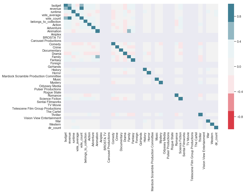
vote_average, my response variable, isn’t highly correlated with any other variable, so there are not currently any stand-out features that I think will be particularly predictive.
Within my features, there are four stronger correlations :
- revenue and budget
- vote_count and budget
- revenue and vote_count
- family and animation
I’ll look at these relationships in greater detail below.
revenue and budget
sns.regplot(x='revenue', y='budget', data=final_dataset_wo_dir)
plt.title('Revenue vs Budget')
plt.xlabel('Revenue')
plt.ylabel('Budget')
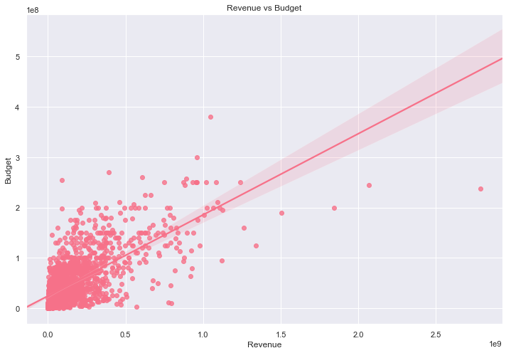
Since the points are very clustered together, I will visualise this a double-log scale to see if I can get a better view of the relationship.
rev_vs_bug = sns.regplot(x='revenue', y='budget', data=final_dataset_wo_dir)
plt.title('Revenue vs Budget')
plt.xlabel('Revenue')
plt.ylabel('Budget')
rev_vs_bug.set(xscale="log", yscale="log")
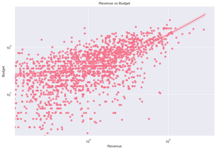
The relationship is strong at 0.69, although it is not represented perfectly by a straight line. The correlation coefficient between revenue and budget. It also makes intuitive sense that movies that have larger budgets will attract larger audiences.
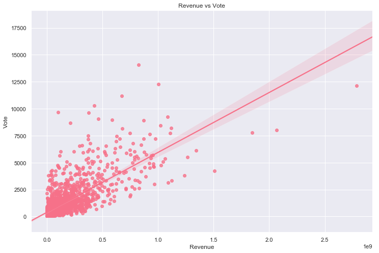
revenue and vote_count
sns.regplot(x='revenue', y='vote_count', data=final_dataset_wo_dir)
plt.title('Revenue vs Vote')
plt.xlabel('Revenue')
plt.ylabel('Vote')
rev_vs_vote = sns.regplot(x='revenue', y='vote_count', data=final_dataset_wo_dir)
plt.title('Revenue vs Vote')
plt.xlabel('Revenue')
plt.ylabel('Vote')
rev_vs_vote.set(xscale="log", yscale="log")

Again, the relationship is better illustrated on a double-log scale and not perfectly represented by a straight line. The correlation coefficient between revenue and vote_count is even more significant at 0.74. As with the relationship between revenue and budget, the larger an audience the higher the number of votes can be expected.
vote_count and budget
sns.regplot(x='budget', y='vote_count', data=final_dataset_wo_dir)
plt.title('Vote Count vs Budget')
plt.xlabel('Budget')
plt.ylabel('Vote Count')

votecount_vs_budget = sns.regplot(x='budget', y='vote_count', data=final_dataset_wo_dir)
plt.title('Vote Count vs Budget')
plt.xlabel('Budget')
plt.ylabel('Vote Count')
votecount_vs_budget.set(xscale="log", yscale="log")
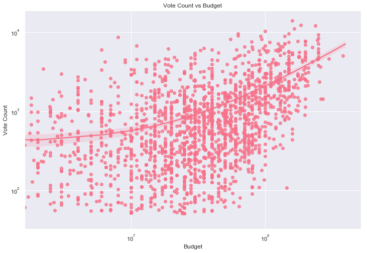
Although there is a correlation coefficient of 0.52, the relationship is again not exactly linear. It appears films with a larger budget spent producing them tend to generate more votes, which makes sense.
Family and Animation
# Both
both = len(final_dataset_wo_dir[(final_dataset_wo_dir['Family'] == 1) & (final_dataset_wo_dir['Animation'] == 1)])

# Animation
ani = len(final_dataset_wo_dir[final_dataset_wo_dir['Animation'] == 1])

# Family
fam = len(final_dataset_wo_dir[final_dataset_wo_dir['Family'] == 1])
venn2(subsets = (fam-both, ani-both, 67),
      set_labels = ('Family', 'Animation'))
plt.show()
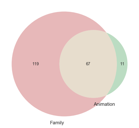
There are, in total, 78 films of genre ‘Animation’ and 186 films of genre ‘Family’. While most Animation films are also classified as Family, the same cannot be said for the other way around. Since this is the case, I will keep both predictors as they are in my models.
The highest and lowest rated films
Highest rated
final_dataset_wo_dir[['title', 'vote_average']].sort_values(by = 'vote_average', ascending = False).head(10)
| title | vote_average | |
|---|---|---|
| 849 | The Godfather | 8.5 |
| 13316 | The Dark Knight | 8.3 |
| 537 | Schindler's List | 8.3 |
| 5766 | Spirited Away | 8.3 |
| 2985 | Fight Club | 8.3 |
| 1199 | One Flew Over the Cuckoo's Nest | 8.3 |
| 300 | Pulp Fiction | 8.3 |
| 1225 | The Godfather: Part II | 8.3 |
| 1223 | Psycho | 8.3 |
| 297 | Leon: The Professional | 8.2 |
Lowest rated
final_dataset_wo_dir[['title', 'vote_average']].sort_values(by = 'vote_average', ascending = True).head(10)
| title | vote_average | |
|---|---|---|
| 13786 | Disaster Movie | 3.1 |
| 12287 | Epic Movie | 3.2 |
| 6795 | Gigli | 3.5 |
| 11468 | Date Movie | 3.6 |
| 13179 | Meet the Spartans | 3.8 |
| 14420 | Street Fighter: The Legend of Chun-Li | 3.9 |
| 19506 | Jack and Jill | 4.0 |
| 22997 | The Canyons | 4.1 |
| 30203 | The Boy Next Door | 4.1 |
| 1557 | Speed 2: Cruise Control | 4.1 |
Dummy variables
As well as making the variables in the final_dataset_wo_dir dummy, I also need to manually add the directors. I’ll do this by creating a pivot table with the directors as columns, the movie id as the row and the values as either 0 or 1.
Since the feature importance of dummy variables relies on the baseline of the first variable that is dropped, I’ll make a note of whom that is in lead, supporting and director for later analysis.
dropped_dummies = final_dataset_wo_dir[['lead', 'supporting']].head(1)
dropped_dummies
| lead | supporting | |
|---|---|---|
| 0 | Tom Hanks | Tim Allen |
dummies = pd.get_dummies(final_dataset_wo_dir, columns=['lead', 'supporting'], drop_first=True)
dummies.head()
| title | id | budget | revenue | runtime | vote_average | vote_count | belongs_to_collection | Action | Adventure | Animation | Aniplex | BROSTA TV | Carousel Productions | Comedy | Crime | Documentary | Drama | Family | Fantasy | Foreign | GoHands | History | Horror | Mardock Scramble Production Committee | Music | Mystery | Odyssey Media | Pulser Productions | Rogue State | Romance | Science Fiction | Sentai Filmworks | TV Movie | Telescene Film Group Productions | The Cartel | Thriller | Vision View Entertainment | War | Western | dir_count | lead_Aaron Eckhart | lead_Aaron Taylor-Johnson | lead_Adam Brody | lead_Adam Sandler | lead_Adrien Brody | lead_Adrienne Barbeau | lead_Aileen Quinn | lead_Al Pacino | lead_Alan Arkin | lead_Alec Baldwin | lead_Alex D. Linz | lead_Alex Frost | lead_Alex Pettyfer | lead_Alexa PenaVega | lead_Alexander Skarsgård | lead_Ali Larter | lead_Alison Lohman | lead_Alyson Hannigan | lead_Amanda Bynes | lead_Amanda Seyfried | lead_Amber Tamblyn | lead_Amber Valletta | lead_Amy Adams | lead_Amy Schumer | lead_Andrew Dice Clay | lead_Andrew Garfield | lead_Andy García | lead_Andy Samberg | lead_Angelina Jolie | lead_Anika Noni Rose | lead_Anna Faris | lead_Anna Kendrick | lead_Anne Hathaway | lead_Ansel Elgort | lead_Anthony Hopkins | lead_Anthony Perkins | lead_Anthony Rapp | lead_Antonio Banderas | lead_Arnold Schwarzenegger | lead_Arthur Hill | lead_Asa Butterfield | lead_Ashley Judd | lead_Ashton Kutcher | lead_Aubrey Peeples | lead_Audrey Hepburn | lead_Audrey Tautou | lead_Auli'i Cravalho | lead_Barbara Harris | lead_Barney Clark | lead_Barret Oliver | lead_Barrie Ingham | lead_Ben Affleck | lead_Ben Kingsley | lead_Ben Stiller | lead_Ben Whishaw | lead_Benedict Cumberbatch | lead_Benicio del Toro | lead_Benjamin Bratt | lead_Benjamin Walker | lead_Bill Murray | lead_Bill Nighy | lead_Bill Pullman | lead_Billy Bob Thornton | lead_Billy Campbell | lead_Billy Crystal | lead_Björk | lead_Blake Jenner | lead_Blake Lively | lead_Bob Hoskins | lead_Bob Newhart | lead_Bobby Campo | lead_Bobby Driscoll | lead_Bodil Jørgensen | lead_Brad Davis | lead_Brad Pitt | lead_Bradley Cooper | lead_Brady Corbet | lead_Brandon Lee | lead_Brandon Routh | lead_Breckin Meyer | lead_Brendan Fraser | lead_Brenton Thwaites | lead_Brian Bedford | lead_Brian O'Halloran | lead_Briana Evigan | lead_Britt Robertson | lead_Bruce Campbell | lead_Bruce Dern | lead_Bruce Reitherman | lead_Bruce Willis | lead_Bryan Cranston | lead_Bryce Dallas Howard | lead_Burt Lancaster | lead_Burt Reynolds | lead_Cameron Diaz | lead_Camilla Belle | lead_Carice van Houten | lead_Carmen Maura | lead_Carroll Baker | lead_Cary Elwes | lead_Cary Grant | lead_Casper Van Dien | lead_Cate Blanchett | lead_Catherine Deneuve | lead_Catherine Zeta-Jones | lead_Cecilia Roth | lead_Chadwick Boseman | lead_Chang Chen | lead_Channing Tatum | lead_Charles Bronson | lead_Charlie Chaplin | lead_Charlie Hunnam | lead_Charlie Sheen | lead_Charlie Tahan | lead_Charlize Theron | lead_Chevy Chase | lead_Chow Yun-fat | lead_Chris Evans | lead_Chris Hemsworth | lead_Chris O'Donnell | lead_Chris Pine | lead_Chris Riggi | lead_Chris Rock | lead_Chris Tucker | lead_Christian Bale | lead_Christian Slater | lead_Christina Applegate | lead_Christina Ricci | lead_Christine Hargreaves | lead_Christoph Waltz | lead_Christopher Guest | lead_Christopher Lambert | lead_Christopher Plummer | lead_Christopher Reeve | lead_Christopher Walken | lead_Cillian Murphy | lead_Claire Danes | lead_Claire Trevor | lead_Clark Gable | lead_Cleavon Little | lead_Clint Eastwood | lead_Clive Owen | lead_Colin Farrell | lead_Colin Firth | lead_Craig T. Nelson | lead_Craig Wasson | lead_Cuba Gooding Jr. | lead_Daisy Ridley | lead_Dakota Blue Richards | lead_Dakota Johnson | lead_Dan Aykroyd | lead_Dane DeHaan | lead_Daniel Brühl | lead_Daniel Craig | lead_Daniel Day-Lewis | lead_Daniel Radcliffe | lead_Danny Aiello | lead_Danny DeVito | lead_Danny McBride | lead_Danny Trejo | lead_Dany Boon | lead_David Arquette | lead_David Duchovny | lead_David Emge | lead_David Naughton | lead_David Niven | lead_David Strathairn | lead_Debra Winger | lead_Dee Wallace | lead_Demi Moore | lead_Demián Bichir | lead_Dennis Quaid | lead_Denzel Washington | lead_Derek Jacobi | lead_Derek Luke | lead_Dev Patel | lead_Diana Ross | lead_Dominic Cooper | lead_Dominique Pinon | lead_Donald Pleasence | lead_Donald Sutherland | lead_Drew Barrymore | lead_Duane Jones | lead_Dustin Hoffman | lead_Dwayne Johnson | lead_Ed Harris | lead_Eddie Griffin | lead_Eddie Murphy | lead_Eddie Redmayne | lead_Edmund Gwenn | lead_Eduardo Noriega | lead_Edward Norton | lead_Eli Marienthal | lead_Elijah Wood | lead_Elisha Cuthbert | lead_Elizabeth Berkley | lead_Elizabeth Hurley | lead_Elizabeth Taylor | lead_Ellar Coltrane | lead_Elle Fanning | lead_Ellen Burstyn | lead_Ellen Page | lead_Emile Hirsch | lead_Emilio Estevez | lead_Emily Barclay | lead_Emily Blunt | lead_Emily Browning | lead_Emily Watson | lead_Emma Thompson | ... | supporting_Peter Sellers | supporting_Phil Harris | supporting_Phil Hartman | supporting_Philip Seymour Hoffman | supporting_Phoebe Cates | supporting_Pierce Brosnan | supporting_Piper Laurie | supporting_Piper Perabo | supporting_Polly Adams | supporting_Powers Boothe | supporting_Priscilla Presley | supporting_Queen Latifah | supporting_Quentin Tarantino | supporting_Quinton Aaron | supporting_Rachel Griffiths | supporting_Rachel McAdams | supporting_Rachel Nichols | supporting_Rachel Weisz | supporting_Radha Mitchell | supporting_Raini Rodriguez | supporting_Ralph Fiennes | supporting_Ralph Macchio | supporting_Rami Malek | supporting_Randy Quaid | supporting_Raoul Bova | supporting_Raquel Castro | supporting_Raquel Welch | supporting_Ray Allen | supporting_Ray Liotta | supporting_Ray Winstone | supporting_Ray Wise | supporting_Raymond J. Barry | supporting_Rebecca Hall | supporting_Reese Witherspoon | supporting_Regina Hall | supporting_Rei Sakuma | supporting_Rene Russo | supporting_Renée Zellweger | supporting_Rhys Ifans | supporting_Richard Attenborough | supporting_Richard Basehart | supporting_Richard Beymer | supporting_Richard Burton | supporting_Richard Dreyfuss | supporting_Richard Gere | supporting_Richard Kind | supporting_Rick Moranis | supporting_River Phoenix | supporting_Rob Brown | supporting_Robert Carlyle | supporting_Robert De Niro | supporting_Robert Downey Jr. | supporting_Robert Duvall | supporting_Robert Englund | supporting_Robert Hoffman | supporting_Robert Pattinson | supporting_Robert Redford | supporting_Robert Sean Leonard | supporting_Robert Shaw | supporting_Robert Walker | supporting_Roberto Benigni | supporting_Robin Shou | supporting_Robin Tunney | supporting_Robin Williams | supporting_Robin Wright | supporting_Rochelle Davis | supporting_Rod Taylor | supporting_Rodney Dangerfield | supporting_Roger B. Smith | supporting_Ron Howard | supporting_Ron Perlman | supporting_Ronee Blakley | supporting_Rooney Mara | supporting_Rory Cochrane | supporting_Rosamund Pike | supporting_Rosanna Arquette | supporting_Rosario Dawson | supporting_Rosario Flores | supporting_Rose Byrne | supporting_Rufus Sewell | supporting_Rupert Grint | supporting_Russell Brand | supporting_Russell Crowe | supporting_Rutger Hauer | supporting_Ryan Gosling | supporting_Ryan Guzman | supporting_Ryan Reynolds | supporting_Sacha Baron Cohen | supporting_Saffron Burrows | supporting_Sally Field | supporting_Salma Hayek | supporting_Sam Neill | supporting_Sam Rockwell | supporting_Sam Worthington | supporting_Samaire Armstrong | supporting_Samuel L. Jackson | supporting_Sandra Bullock | supporting_Sarah Berry | supporting_Sarah Michelle Gellar | supporting_Sarah Roemer | supporting_Sarita Choudhury | supporting_Scarlett Johansson | supporting_Scott Bakula | supporting_Scott Caan | supporting_Scott MacDonald | supporting_Scott Speedman | supporting_Sean Bean | supporting_Sean Connery | supporting_Sean Penn | supporting_Sean Young | supporting_Seann William Scott | supporting_Sebastian Koch | supporting_Selma Blair | supporting_Seth Green | supporting_Seth Rogen | supporting_Shailene Woodley | supporting_Shane West | supporting_Shannyn Sossamon | supporting_Shantel VanSanten | supporting_Sharon Stone | supporting_Shawnee Smith | supporting_Shelley Duvall | supporting_Sheri Moon Zombie | supporting_Shia LaBeouf | supporting_Shirley MacLaine | supporting_Shu Qi | supporting_Sienna Guillory | supporting_Sienna Miller | supporting_Sigourney Weaver | supporting_Simon Chandler | supporting_Sofía Vergara | supporting_Sondra Locke | supporting_Sonja Smits | supporting_Sophia Myles | supporting_Sophie Marceau | supporting_Soren Fulton | supporting_Spencer Breslin | supporting_Stacy Keach | supporting_Stanley Tucci | supporting_Stefanie Scott | supporting_Stephen Baldwin | supporting_Stephen Rea | supporting_Sterling Holloway | supporting_Steve Carell | supporting_Steve Coogan | supporting_Steve Martin | supporting_Steve Zahn | supporting_Steven Bauer | supporting_Sue Lyon | supporting_Sung Kang | supporting_Susan George | supporting_Susan Sarandon | supporting_Sylvester Stallone | supporting_Sô Yamamura | supporting_T.R. Knight | supporting_Takeshi Kaneshiro | supporting_Talia Shire | supporting_Tara Morice | supporting_Taraji P. Henson | supporting_Taylor Dooley | supporting_Taylor Kitsch | supporting_Taylor Momsen | supporting_Tencho Gyalpo | supporting_Terence Stamp | supporting_Teresa Palmer | supporting_Teri Polo | supporting_Terrence Howard | supporting_Terry Alexander | supporting_Thandie Newton | supporting_Theo James | supporting_Thomas Haden Church | supporting_Thomas Kretschmann | supporting_Thora Birch | supporting_Tim Allen | supporting_Tim Matheson | supporting_Tim Robbins | supporting_Tim Roth | supporting_Timothy Olyphant | supporting_Tina Fey | supporting_Tina Turner | supporting_Tobey Maguire | supporting_Toby Kebbell | supporting_Tom Cruise | supporting_Tom Glynn-Carney | supporting_Tom Hanks | supporting_Tom Hardy | supporting_Tom Hulce | supporting_Tom Sizemore | supporting_Tom Wilkinson | supporting_Tommy Lee Jones | supporting_Toni Collette | supporting_Tony Curtis | supporting_Tony Revolori | supporting_Tracy Morgan | supporting_Tuesday Knight | supporting_Tye Sheridan | supporting_Tyler Hoechlin | supporting_Tyrese Gibson | supporting_Téa Leoni | supporting_Uma Thurman | supporting_Unax Ugalde | supporting_Val Bettin | supporting_Val Kilmer | supporting_Vanessa Bauche | supporting_Vanessa Lachey | supporting_Vera Farmiga | supporting_Vera Miles | supporting_Verna Bloom | supporting_Verna Felton | supporting_Viggo Mortensen | supporting_Vin Diesel | supporting_Vince Vaughn | supporting_Vincent Cassel | supporting_Vincent D'Onofrio | supporting_Vincent Piazza | supporting_Ving Rhames | supporting_Virginia Cherrill | supporting_Virginia Madsen | supporting_Vladimir Kulich | supporting_Vladimir Menshov | supporting_Walter Huston | supporting_Wayne Newton | supporting_Wendy Raquel Robinson | supporting_Wentworth Miller | supporting_Wesley Snipes | supporting_Whitney Houston | supporting_Will Ferrell | supporting_Will Forte | supporting_Will Sasso | supporting_Will Smith | supporting_Willem Dafoe | supporting_William Atherton | supporting_William Baldwin | supporting_William Forsythe | supporting_William H. Macy | supporting_William Holden | supporting_William Hurt | supporting_Winona Ryder | supporting_Woody Harrelson | supporting_Yaphet Kotto | supporting_Yasiin Bey | supporting_Yuriko Ishida | supporting_Zac Efron | supporting_Zach Galifianakis | supporting_Zachary Quinto | supporting_Zoe Saldana | supporting_Zooey Deschanel | supporting_Zoë Bell | supporting_Zuleikha Robinson | supporting_Óscar Jaenada | |
|---|---|---|---|---|---|---|---|---|---|---|---|---|---|---|---|---|---|---|---|---|---|---|---|---|---|---|---|---|---|---|---|---|---|---|---|---|---|---|---|---|---|---|---|---|---|---|---|---|---|---|---|---|---|---|---|---|---|---|---|---|---|---|---|---|---|---|---|---|---|---|---|---|---|---|---|---|---|---|---|---|---|---|---|---|---|---|---|---|---|---|---|---|---|---|---|---|---|---|---|---|---|---|---|---|---|---|---|---|---|---|---|---|---|---|---|---|---|---|---|---|---|---|---|---|---|---|---|---|---|---|---|---|---|---|---|---|---|---|---|---|---|---|---|---|---|---|---|---|---|---|---|---|---|---|---|---|---|---|---|---|---|---|---|---|---|---|---|---|---|---|---|---|---|---|---|---|---|---|---|---|---|---|---|---|---|---|---|---|---|---|---|---|---|---|---|---|---|---|---|---|---|---|---|---|---|---|---|---|---|---|---|---|---|---|---|---|---|---|---|---|---|---|---|---|---|---|---|---|---|---|---|---|---|---|---|---|---|---|---|---|---|---|---|---|---|---|---|---|---|---|---|---|---|---|---|---|---|---|---|---|---|---|---|---|---|---|---|---|---|---|---|---|---|---|---|---|---|---|---|---|---|---|---|---|---|---|---|---|---|---|---|---|---|---|---|---|---|---|---|---|---|---|---|---|---|---|---|---|---|---|---|---|---|---|---|---|---|---|---|---|---|---|---|---|---|---|---|---|---|---|---|---|---|---|---|---|---|---|---|---|---|---|---|---|---|---|---|---|---|---|---|---|---|---|---|---|---|---|---|---|---|---|---|---|---|---|---|---|---|---|---|---|---|---|---|---|---|---|---|---|---|---|---|---|---|---|---|---|---|---|---|---|---|---|---|---|---|---|---|---|---|---|---|---|---|---|---|---|---|---|---|---|---|---|---|---|---|---|---|---|---|---|---|---|---|---|---|---|---|---|---|---|---|---|---|---|---|---|---|---|---|---|---|---|---|---|---|---|---|---|---|---|---|---|---|---|---|---|---|---|---|---|---|---|---|---|---|---|---|---|---|---|---|---|---|---|---|---|---|---|---|---|---|---|---|---|---|---|---|---|---|---|---|---|---|---|---|---|---|---|---|
| 0 | Toy Story | 862 | 30000000.0 | 373554033.0 | 81.0 | 7.7 | 5415.0 | 1 | 0.0 | 0.0 | 1.0 | 0.0 | 0.0 | 0.0 | 1.0 | 0.0 | 0.0 | 0.0 | 1.0 | 0.0 | 0.0 | 0.0 | 0.0 | 0.0 | 0.0 | 0.0 | 0.0 | 0.0 | 0.0 | 0.0 | 0.0 | 0.0 | 0.0 | 0.0 | 0.0 | 0.0 | 0.0 | 0.0 | 0.0 | 0.0 | 5 | 0 | 0 | 0 | 0 | 0 | 0 | 0 | 0 | 0 | 0 | 0 | 0 | 0 | 0 | 0 | 0 | 0 | 0 | 0 | 0 | 0 | 0 | 0 | 0 | 0 | 0 | 0 | 0 | 0 | 0 | 0 | 0 | 0 | 0 | 0 | 0 | 0 | 0 | 0 | 0 | 0 | 0 | 0 | 0 | 0 | 0 | 0 | 0 | 0 | 0 | 0 | 0 | 0 | 0 | 0 | 0 | 0 | 0 | 0 | 0 | 0 | 0 | 0 | 0 | 0 | 0 | 0 | 0 | 0 | 0 | 0 | 0 | 0 | 0 | 0 | 0 | 0 | 0 | 0 | 0 | 0 | 0 | 0 | 0 | 0 | 0 | 0 | 0 | 0 | 0 | 0 | 0 | 0 | 0 | 0 | 0 | 0 | 0 | 0 | 0 | 0 | 0 | 0 | 0 | 0 | 0 | 0 | 0 | 0 | 0 | 0 | 0 | 0 | 0 | 0 | 0 | 0 | 0 | 0 | 0 | 0 | 0 | 0 | 0 | 0 | 0 | 0 | 0 | 0 | 0 | 0 | 0 | 0 | 0 | 0 | 0 | 0 | 0 | 0 | 0 | 0 | 0 | 0 | 0 | 0 | 0 | 0 | 0 | 0 | 0 | 0 | 0 | 0 | 0 | 0 | 0 | 0 | 0 | 0 | 0 | 0 | 0 | 0 | 0 | 0 | 0 | 0 | 0 | 0 | 0 | 0 | 0 | 0 | 0 | 0 | 0 | 0 | 0 | 0 | 0 | 0 | 0 | 0 | 0 | 0 | 0 | 0 | 0 | 0 | 0 | 0 | 0 | 0 | 0 | 0 | 0 | 0 | 0 | 0 | 0 | 0 | 0 | 0 | 0 | 0 | 0 | 0 | 0 | 0 | ... | 0 | 0 | 0 | 0 | 0 | 0 | 0 | 0 | 0 | 0 | 0 | 0 | 0 | 0 | 0 | 0 | 0 | 0 | 0 | 0 | 0 | 0 | 0 | 0 | 0 | 0 | 0 | 0 | 0 | 0 | 0 | 0 | 0 | 0 | 0 | 0 | 0 | 0 | 0 | 0 | 0 | 0 | 0 | 0 | 0 | 0 | 0 | 0 | 0 | 0 | 0 | 0 | 0 | 0 | 0 | 0 | 0 | 0 | 0 | 0 | 0 | 0 | 0 | 0 | 0 | 0 | 0 | 0 | 0 | 0 | 0 | 0 | 0 | 0 | 0 | 0 | 0 | 0 | 0 | 0 | 0 | 0 | 0 | 0 | 0 | 0 | 0 | 0 | 0 | 0 | 0 | 0 | 0 | 0 | 0 | 0 | 0 | 0 | 0 | 0 | 0 | 0 | 0 | 0 | 0 | 0 | 0 | 0 | 0 | 0 | 0 | 0 | 0 | 0 | 0 | 0 | 0 | 0 | 0 | 0 | 0 | 0 | 0 | 0 | 0 | 0 | 0 | 0 | 0 | 0 | 0 | 0 | 0 | 0 | 0 | 0 | 0 | 0 | 0 | 0 | 0 | 0 | 0 | 0 | 0 | 0 | 0 | 0 | 0 | 0 | 0 | 0 | 0 | 0 | 0 | 0 | 0 | 0 | 0 | 0 | 0 | 0 | 0 | 0 | 0 | 0 | 0 | 0 | 0 | 0 | 0 | 0 | 0 | 1 | 0 | 0 | 0 | 0 | 0 | 0 | 0 | 0 | 0 | 0 | 0 | 0 | 0 | 0 | 0 | 0 | 0 | 0 | 0 | 0 | 0 | 0 | 0 | 0 | 0 | 0 | 0 | 0 | 0 | 0 | 0 | 0 | 0 | 0 | 0 | 0 | 0 | 0 | 0 | 0 | 0 | 0 | 0 | 0 | 0 | 0 | 0 | 0 | 0 | 0 | 0 | 0 | 0 | 0 | 0 | 0 | 0 | 0 | 0 | 0 | 0 | 0 | 0 | 0 | 0 | 0 | 0 | 0 | 0 | 0 | 0 | 0 | 0 | 0 | 0 | 0 |
| 1 | Jumanji | 8844 | 65000000.0 | 262797249.0 | 104.0 | 6.9 | 2413.0 | 0 | 0.0 | 1.0 | 0.0 | 0.0 | 0.0 | 0.0 | 0.0 | 0.0 | 0.0 | 0.0 | 1.0 | 1.0 | 0.0 | 0.0 | 0.0 | 0.0 | 0.0 | 0.0 | 0.0 | 0.0 | 0.0 | 0.0 | 0.0 | 0.0 | 0.0 | 0.0 | 0.0 | 0.0 | 0.0 | 0.0 | 0.0 | 0.0 | 7 | 0 | 0 | 0 | 0 | 0 | 0 | 0 | 0 | 0 | 0 | 0 | 0 | 0 | 0 | 0 | 0 | 0 | 0 | 0 | 0 | 0 | 0 | 0 | 0 | 0 | 0 | 0 | 0 | 0 | 0 | 0 | 0 | 0 | 0 | 0 | 0 | 0 | 0 | 0 | 0 | 0 | 0 | 0 | 0 | 0 | 0 | 0 | 0 | 0 | 0 | 0 | 0 | 0 | 0 | 0 | 0 | 0 | 0 | 0 | 0 | 0 | 0 | 0 | 0 | 0 | 0 | 0 | 0 | 0 | 0 | 0 | 0 | 0 | 0 | 0 | 0 | 0 | 0 | 0 | 0 | 0 | 0 | 0 | 0 | 0 | 0 | 0 | 0 | 0 | 0 | 0 | 0 | 0 | 0 | 0 | 0 | 0 | 0 | 0 | 0 | 0 | 0 | 0 | 0 | 0 | 0 | 0 | 0 | 0 | 0 | 0 | 0 | 0 | 0 | 0 | 0 | 0 | 0 | 0 | 0 | 0 | 0 | 0 | 0 | 0 | 0 | 0 | 0 | 0 | 0 | 0 | 0 | 0 | 0 | 0 | 0 | 0 | 0 | 0 | 0 | 0 | 0 | 0 | 0 | 0 | 0 | 0 | 0 | 0 | 0 | 0 | 0 | 0 | 0 | 0 | 0 | 0 | 0 | 0 | 0 | 0 | 0 | 0 | 0 | 0 | 0 | 0 | 0 | 0 | 0 | 0 | 0 | 0 | 0 | 0 | 0 | 0 | 0 | 0 | 0 | 0 | 0 | 0 | 0 | 0 | 0 | 0 | 0 | 0 | 0 | 0 | 0 | 0 | 0 | 0 | 0 | 0 | 0 | 0 | 0 | 0 | 0 | 0 | 0 | 0 | 0 | 0 | 0 | 0 | ... | 0 | 0 | 0 | 0 | 0 | 0 | 0 | 0 | 0 | 0 | 0 | 0 | 0 | 0 | 0 | 0 | 0 | 0 | 0 | 0 | 0 | 0 | 0 | 0 | 0 | 0 | 0 | 0 | 0 | 0 | 0 | 0 | 0 | 0 | 0 | 0 | 0 | 0 | 0 | 0 | 0 | 0 | 0 | 0 | 0 | 0 | 0 | 0 | 0 | 0 | 0 | 0 | 0 | 0 | 0 | 0 | 0 | 0 | 0 | 0 | 0 | 0 | 0 | 0 | 0 | 0 | 0 | 0 | 0 | 0 | 0 | 0 | 0 | 0 | 0 | 0 | 0 | 0 | 0 | 0 | 0 | 0 | 0 | 0 | 0 | 0 | 0 | 0 | 0 | 0 | 0 | 0 | 0 | 0 | 0 | 0 | 0 | 0 | 0 | 0 | 0 | 0 | 0 | 0 | 0 | 0 | 0 | 0 | 0 | 0 | 0 | 0 | 0 | 0 | 0 | 0 | 0 | 0 | 0 | 0 | 0 | 0 | 0 | 0 | 0 | 0 | 0 | 0 | 0 | 0 | 0 | 0 | 0 | 0 | 0 | 0 | 0 | 0 | 0 | 0 | 0 | 0 | 0 | 0 | 0 | 0 | 0 | 0 | 0 | 0 | 0 | 0 | 0 | 0 | 0 | 0 | 0 | 0 | 0 | 0 | 0 | 0 | 0 | 0 | 0 | 0 | 0 | 0 | 0 | 0 | 0 | 0 | 0 | 0 | 0 | 0 | 0 | 0 | 0 | 0 | 0 | 0 | 0 | 0 | 0 | 0 | 0 | 0 | 0 | 0 | 0 | 0 | 0 | 0 | 0 | 0 | 0 | 0 | 0 | 0 | 0 | 0 | 0 | 0 | 0 | 0 | 0 | 0 | 0 | 0 | 0 | 0 | 0 | 0 | 0 | 0 | 0 | 0 | 0 | 0 | 0 | 0 | 0 | 0 | 0 | 0 | 0 | 0 | 0 | 0 | 0 | 0 | 0 | 0 | 0 | 0 | 0 | 0 | 0 | 0 | 0 | 0 | 0 | 0 | 0 | 0 | 0 | 0 | 0 | 0 |
| 5 | Heat | 949 | 60000000.0 | 187436818.0 | 170.0 | 7.7 | 1886.0 | 0 | 1.0 | 0.0 | 0.0 | 0.0 | 0.0 | 0.0 | 0.0 | 1.0 | 0.0 | 1.0 | 0.0 | 0.0 | 0.0 | 0.0 | 0.0 | 0.0 | 0.0 | 0.0 | 0.0 | 0.0 | 0.0 | 0.0 | 0.0 | 0.0 | 0.0 | 0.0 | 0.0 | 0.0 | 1.0 | 0.0 | 0.0 | 0.0 | 10 | 0 | 0 | 0 | 0 | 0 | 0 | 0 | 1 | 0 | 0 | 0 | 0 | 0 | 0 | 0 | 0 | 0 | 0 | 0 | 0 | 0 | 0 | 0 | 0 | 0 | 0 | 0 | 0 | 0 | 0 | 0 | 0 | 0 | 0 | 0 | 0 | 0 | 0 | 0 | 0 | 0 | 0 | 0 | 0 | 0 | 0 | 0 | 0 | 0 | 0 | 0 | 0 | 0 | 0 | 0 | 0 | 0 | 0 | 0 | 0 | 0 | 0 | 0 | 0 | 0 | 0 | 0 | 0 | 0 | 0 | 0 | 0 | 0 | 0 | 0 | 0 | 0 | 0 | 0 | 0 | 0 | 0 | 0 | 0 | 0 | 0 | 0 | 0 | 0 | 0 | 0 | 0 | 0 | 0 | 0 | 0 | 0 | 0 | 0 | 0 | 0 | 0 | 0 | 0 | 0 | 0 | 0 | 0 | 0 | 0 | 0 | 0 | 0 | 0 | 0 | 0 | 0 | 0 | 0 | 0 | 0 | 0 | 0 | 0 | 0 | 0 | 0 | 0 | 0 | 0 | 0 | 0 | 0 | 0 | 0 | 0 | 0 | 0 | 0 | 0 | 0 | 0 | 0 | 0 | 0 | 0 | 0 | 0 | 0 | 0 | 0 | 0 | 0 | 0 | 0 | 0 | 0 | 0 | 0 | 0 | 0 | 0 | 0 | 0 | 0 | 0 | 0 | 0 | 0 | 0 | 0 | 0 | 0 | 0 | 0 | 0 | 0 | 0 | 0 | 0 | 0 | 0 | 0 | 0 | 0 | 0 | 0 | 0 | 0 | 0 | 0 | 0 | 0 | 0 | 0 | 0 | 0 | 0 | 0 | 0 | 0 | 0 | 0 | 0 | 0 | 0 | 0 | 0 | 0 | ... | 0 | 0 | 0 | 0 | 0 | 0 | 0 | 0 | 0 | 0 | 0 | 0 | 0 | 0 | 0 | 0 | 0 | 0 | 0 | 0 | 0 | 0 | 0 | 0 | 0 | 0 | 0 | 0 | 0 | 0 | 0 | 0 | 0 | 0 | 0 | 0 | 0 | 0 | 0 | 0 | 0 | 0 | 0 | 0 | 0 | 0 | 0 | 0 | 0 | 0 | 1 | 0 | 0 | 0 | 0 | 0 | 0 | 0 | 0 | 0 | 0 | 0 | 0 | 0 | 0 | 0 | 0 | 0 | 0 | 0 | 0 | 0 | 0 | 0 | 0 | 0 | 0 | 0 | 0 | 0 | 0 | 0 | 0 | 0 | 0 | 0 | 0 | 0 | 0 | 0 | 0 | 0 | 0 | 0 | 0 | 0 | 0 | 0 | 0 | 0 | 0 | 0 | 0 | 0 | 0 | 0 | 0 | 0 | 0 | 0 | 0 | 0 | 0 | 0 | 0 | 0 | 0 | 0 | 0 | 0 | 0 | 0 | 0 | 0 | 0 | 0 | 0 | 0 | 0 | 0 | 0 | 0 | 0 | 0 | 0 | 0 | 0 | 0 | 0 | 0 | 0 | 0 | 0 | 0 | 0 | 0 | 0 | 0 | 0 | 0 | 0 | 0 | 0 | 0 | 0 | 0 | 0 | 0 | 0 | 0 | 0 | 0 | 0 | 0 | 0 | 0 | 0 | 0 | 0 | 0 | 0 | 0 | 0 | 0 | 0 | 0 | 0 | 0 | 0 | 0 | 0 | 0 | 0 | 0 | 0 | 0 | 0 | 0 | 0 | 0 | 0 | 0 | 0 | 0 | 0 | 0 | 0 | 0 | 0 | 0 | 0 | 0 | 0 | 0 | 0 | 0 | 0 | 0 | 0 | 0 | 0 | 0 | 0 | 0 | 0 | 0 | 0 | 0 | 0 | 0 | 0 | 0 | 0 | 0 | 0 | 0 | 0 | 0 | 0 | 0 | 0 | 0 | 0 | 0 | 0 | 0 | 0 | 0 | 0 | 0 | 0 | 0 | 0 | 0 | 0 | 0 | 0 | 0 | 0 | 0 |
| 8 | Sudden Death | 9091 | 35000000.0 | 64350171.0 | 106.0 | 5.5 | 174.0 | 0 | 1.0 | 1.0 | 0.0 | 0.0 | 0.0 | 0.0 | 0.0 | 0.0 | 0.0 | 0.0 | 0.0 | 0.0 | 0.0 | 0.0 | 0.0 | 0.0 | 0.0 | 0.0 | 0.0 | 0.0 | 0.0 | 0.0 | 0.0 | 0.0 | 0.0 | 0.0 | 0.0 | 0.0 | 1.0 | 0.0 | 0.0 | 0.0 | 10 | 0 | 0 | 0 | 0 | 0 | 0 | 0 | 0 | 0 | 0 | 0 | 0 | 0 | 0 | 0 | 0 | 0 | 0 | 0 | 0 | 0 | 0 | 0 | 0 | 0 | 0 | 0 | 0 | 0 | 0 | 0 | 0 | 0 | 0 | 0 | 0 | 0 | 0 | 0 | 0 | 0 | 0 | 0 | 0 | 0 | 0 | 0 | 0 | 0 | 0 | 0 | 0 | 0 | 0 | 0 | 0 | 0 | 0 | 0 | 0 | 0 | 0 | 0 | 0 | 0 | 0 | 0 | 0 | 0 | 0 | 0 | 0 | 0 | 0 | 0 | 0 | 0 | 0 | 0 | 0 | 0 | 0 | 0 | 0 | 0 | 0 | 0 | 0 | 0 | 0 | 0 | 0 | 0 | 0 | 0 | 0 | 0 | 0 | 0 | 0 | 0 | 0 | 0 | 0 | 0 | 0 | 0 | 0 | 0 | 0 | 0 | 0 | 0 | 0 | 0 | 0 | 0 | 0 | 0 | 0 | 0 | 0 | 0 | 0 | 0 | 0 | 0 | 0 | 0 | 0 | 0 | 0 | 0 | 0 | 0 | 0 | 0 | 0 | 0 | 0 | 0 | 0 | 0 | 0 | 0 | 0 | 0 | 0 | 0 | 0 | 0 | 0 | 0 | 0 | 0 | 0 | 0 | 0 | 0 | 0 | 0 | 0 | 0 | 0 | 0 | 0 | 0 | 0 | 0 | 0 | 0 | 0 | 0 | 0 | 0 | 0 | 0 | 0 | 0 | 0 | 0 | 0 | 0 | 0 | 0 | 0 | 0 | 0 | 0 | 0 | 0 | 0 | 0 | 0 | 0 | 0 | 0 | 0 | 0 | 0 | 0 | 0 | 0 | 0 | 0 | 0 | 0 | 0 | 0 | ... | 0 | 0 | 0 | 0 | 0 | 0 | 0 | 0 | 0 | 1 | 0 | 0 | 0 | 0 | 0 | 0 | 0 | 0 | 0 | 0 | 0 | 0 | 0 | 0 | 0 | 0 | 0 | 0 | 0 | 0 | 0 | 0 | 0 | 0 | 0 | 0 | 0 | 0 | 0 | 0 | 0 | 0 | 0 | 0 | 0 | 0 | 0 | 0 | 0 | 0 | 0 | 0 | 0 | 0 | 0 | 0 | 0 | 0 | 0 | 0 | 0 | 0 | 0 | 0 | 0 | 0 | 0 | 0 | 0 | 0 | 0 | 0 | 0 | 0 | 0 | 0 | 0 | 0 | 0 | 0 | 0 | 0 | 0 | 0 | 0 | 0 | 0 | 0 | 0 | 0 | 0 | 0 | 0 | 0 | 0 | 0 | 0 | 0 | 0 | 0 | 0 | 0 | 0 | 0 | 0 | 0 | 0 | 0 | 0 | 0 | 0 | 0 | 0 | 0 | 0 | 0 | 0 | 0 | 0 | 0 | 0 | 0 | 0 | 0 | 0 | 0 | 0 | 0 | 0 | 0 | 0 | 0 | 0 | 0 | 0 | 0 | 0 | 0 | 0 | 0 | 0 | 0 | 0 | 0 | 0 | 0 | 0 | 0 | 0 | 0 | 0 | 0 | 0 | 0 | 0 | 0 | 0 | 0 | 0 | 0 | 0 | 0 | 0 | 0 | 0 | 0 | 0 | 0 | 0 | 0 | 0 | 0 | 0 | 0 | 0 | 0 | 0 | 0 | 0 | 0 | 0 | 0 | 0 | 0 | 0 | 0 | 0 | 0 | 0 | 0 | 0 | 0 | 0 | 0 | 0 | 0 | 0 | 0 | 0 | 0 | 0 | 0 | 0 | 0 | 0 | 0 | 0 | 0 | 0 | 0 | 0 | 0 | 0 | 0 | 0 | 0 | 0 | 0 | 0 | 0 | 0 | 0 | 0 | 0 | 0 | 0 | 0 | 0 | 0 | 0 | 0 | 0 | 0 | 0 | 0 | 0 | 0 | 0 | 0 | 0 | 0 | 0 | 0 | 0 | 0 | 0 | 0 | 0 | 0 | 0 |
| 9 | GoldenEye | 710 | 58000000.0 | 352194034.0 | 130.0 | 6.6 | 1194.0 | 1 | 1.0 | 1.0 | 0.0 | 0.0 | 0.0 | 0.0 | 0.0 | 0.0 | 0.0 | 0.0 | 0.0 | 0.0 | 0.0 | 0.0 | 0.0 | 0.0 | 0.0 | 0.0 | 0.0 | 0.0 | 0.0 | 0.0 | 0.0 | 0.0 | 0.0 | 0.0 | 0.0 | 0.0 | 1.0 | 0.0 | 0.0 | 0.0 | 8 | 0 | 0 | 0 | 0 | 0 | 0 | 0 | 0 | 0 | 0 | 0 | 0 | 0 | 0 | 0 | 0 | 0 | 0 | 0 | 0 | 0 | 0 | 0 | 0 | 0 | 0 | 0 | 0 | 0 | 0 | 0 | 0 | 0 | 0 | 0 | 0 | 0 | 0 | 0 | 0 | 0 | 0 | 0 | 0 | 0 | 0 | 0 | 0 | 0 | 0 | 0 | 0 | 0 | 0 | 0 | 0 | 0 | 0 | 0 | 0 | 0 | 0 | 0 | 0 | 0 | 0 | 0 | 0 | 0 | 0 | 0 | 0 | 0 | 0 | 0 | 0 | 0 | 0 | 0 | 0 | 0 | 0 | 0 | 0 | 0 | 0 | 0 | 0 | 0 | 0 | 0 | 0 | 0 | 0 | 0 | 0 | 0 | 0 | 0 | 0 | 0 | 0 | 0 | 0 | 0 | 0 | 0 | 0 | 0 | 0 | 0 | 0 | 0 | 0 | 0 | 0 | 0 | 0 | 0 | 0 | 0 | 0 | 0 | 0 | 0 | 0 | 0 | 0 | 0 | 0 | 0 | 0 | 0 | 0 | 0 | 0 | 0 | 0 | 0 | 0 | 0 | 0 | 0 | 0 | 0 | 0 | 0 | 0 | 0 | 0 | 0 | 0 | 0 | 0 | 0 | 0 | 0 | 0 | 0 | 0 | 0 | 0 | 0 | 0 | 0 | 0 | 0 | 0 | 0 | 0 | 0 | 0 | 0 | 0 | 0 | 0 | 0 | 0 | 0 | 0 | 0 | 0 | 0 | 0 | 0 | 0 | 0 | 0 | 0 | 0 | 0 | 0 | 0 | 0 | 0 | 0 | 0 | 0 | 0 | 0 | 0 | 0 | 0 | 0 | 0 | 0 | 0 | 0 | 0 | ... | 0 | 0 | 0 | 0 | 0 | 0 | 0 | 0 | 0 | 0 | 0 | 0 | 0 | 0 | 0 | 0 | 0 | 0 | 0 | 0 | 0 | 0 | 0 | 0 | 0 | 0 | 0 | 0 | 0 | 0 | 0 | 0 | 0 | 0 | 0 | 0 | 0 | 0 | 0 | 0 | 0 | 0 | 0 | 0 | 0 | 0 | 0 | 0 | 0 | 0 | 0 | 0 | 0 | 0 | 0 | 0 | 0 | 0 | 0 | 0 | 0 | 0 | 0 | 0 | 0 | 0 | 0 | 0 | 0 | 0 | 0 | 0 | 0 | 0 | 0 | 0 | 0 | 0 | 0 | 0 | 0 | 0 | 0 | 0 | 0 | 0 | 0 | 0 | 0 | 0 | 0 | 0 | 0 | 0 | 0 | 0 | 0 | 0 | 0 | 0 | 0 | 0 | 0 | 0 | 0 | 0 | 1 | 0 | 0 | 0 | 0 | 0 | 0 | 0 | 0 | 0 | 0 | 0 | 0 | 0 | 0 | 0 | 0 | 0 | 0 | 0 | 0 | 0 | 0 | 0 | 0 | 0 | 0 | 0 | 0 | 0 | 0 | 0 | 0 | 0 | 0 | 0 | 0 | 0 | 0 | 0 | 0 | 0 | 0 | 0 | 0 | 0 | 0 | 0 | 0 | 0 | 0 | 0 | 0 | 0 | 0 | 0 | 0 | 0 | 0 | 0 | 0 | 0 | 0 | 0 | 0 | 0 | 0 | 0 | 0 | 0 | 0 | 0 | 0 | 0 | 0 | 0 | 0 | 0 | 0 | 0 | 0 | 0 | 0 | 0 | 0 | 0 | 0 | 0 | 0 | 0 | 0 | 0 | 0 | 0 | 0 | 0 | 0 | 0 | 0 | 0 | 0 | 0 | 0 | 0 | 0 | 0 | 0 | 0 | 0 | 0 | 0 | 0 | 0 | 0 | 0 | 0 | 0 | 0 | 0 | 0 | 0 | 0 | 0 | 0 | 0 | 0 | 0 | 0 | 0 | 0 | 0 | 0 | 0 | 0 | 0 | 0 | 0 | 0 | 0 | 0 | 0 | 0 | 0 | 0 |
5 rows × 1847 columns
directors.drop_duplicates(inplace=True)
directors["value"] = 1
unique_dir_names = list(set(directors.director))
master = pd.DataFrame(columns=unique_dir_names)

for n in list(set(directors.id)):
    t = directors[directors["id"] == n]
    pivoted = t.pivot(index="id", columns="director", values="value")
    master = master.append(pivoted)
master.fillna(0, inplace=True)
master.reset_index(level=0, inplace=True)
final = pd.merge(master, dummies, left_on = 'index', right_on = 'id')
Finally, I’ll drop the first director as a reference, as well as the index and id columns used for joining. The director I am dropping is “Aaron Seltzer”, which is worth noting for when I interpret the coefficients.
final.drop(["id", "index", "Aaron Seltzer", "dir_count", "title"], axis=1, inplace=True)
final.drop_duplicates(inplace=True)
master.to_csv("director_dummies.csv")
Pre-processing
Since the final product of this modelling is to produce a Flask app that allows someone to input factors about a film before it’s produced to get the rating and the revenue generated, some features will have to be dropped. For example, a user would not know the vote_count before the film is created. Some of the features I am removing are the most correlated with the response variable so I will be losing some of the predictive power.
I’ll begin by defining my train/test split. Then I’ll standardise the remaining predictive variables since it’s good practice for working with linear regressions. I’ll fit and transform the scaling on my training set and transform on my testing set.
X = final.drop(["vote_average", "revenue", "vote_count"], axis=1)
y = final.vote_average
scaler = StandardScaler()
X_train, X_test, y_train, y_test = ms.train_test_split(X, y, test_size=0.3, random_state=42)
X_train = pd.DataFrame(scaler.fit_transform(X_train), columns=X.columns)
X_test = pd.DataFrame(scaler.transform(X_test), columns=X.columns)
print("Length of training sets:",len(X_train), len(X_test))
print("Length of testing sets:",len(y_train), len(y_test))
Length of training sets: 1296 556
Length of testing sets: 1296 556
Modelling
Baseline score
I need a baseline score with which to compare the scores for all my models moving forward. This score will represent the score one would get if they were just to predict the mean value for y. If my model outperforms this score, I know it is doing well.
y_pred_mean = [y_train.mean()] * len(y_test)

print("Baseline score RMSE: ",'{0:0.2f}'.format(np.sqrt(metrics.mean_squared_error(y_test, y_pred_mean))))
Baseline score RMSE: 0.83
The baseline score is an RMSE of 0.83, meaning that the predicted score is within 0.83 of a mark out of 10. I’ll use this is a benchmark as to the performance of my models.
Ultimately, I will be choosing the model that has the best cross-validated score of all as this will be the one that generalises well. I will also take into account the training and test scores, since these will indicate over or underfitting.
Function to generate model scores
Since I’ll be trying out many different models, I’ll build a function that returns all the information for efficiency. I’ll create one function for simple models and another for models utilising regularisation.
# Function to return simple model metrics
def get_model_metrics(X_train, y_train, X_test, y_test, model, parametric=True):
    """This function takes the train-test splits as arguments, as well as the algorithm
    being used, and returns the training score, the test score (both RMSE), the
    cross-validated scores and the mean cross-validated score. It also returns the appropriate
    feature importances depending on whether the optional argument 'parametric' is equal to
    True or False."""

    model.fit(X_train, y_train)
    train_pred = np.around(model.predict(X_train),1)
    test_pred = np.around(model.predict(X_test),1)

    print('Training score', '{0:0.2f}'.format(np.sqrt(metrics.mean_squared_error(y_train, train_pred))))
    print('Testing RMSE:', '{0:0.2f}'.format(np.sqrt(metrics.mean_squared_error(y_test, test_pred))))
    cv_scores = -ms.cross_val_score(model, X_train, y_train, cv=5, scoring='neg_mean_squared_error')
    print('Cross-validated RMSEs:', np.sqrt(cv_scores))
    print('Mean cross-validated RMSE:', '{0:0.2f}'.format(np.sqrt(np.mean(cv_scores))))

    if parametric == True:
        print(pd.DataFrame(list(zip(X_train.columns, model.coef_, abs(model.coef_))),
                 columns=['Feature', 'Coef', 'Abs Coef']).sort_values('Abs Coef', ascending=False).head(10))
    else:
        print(pd.DataFrame(list(zip(X_train.columns, model.feature_importances_)),
                 columns=['Feature', 'Importance']).sort_values('Importance', ascending=False).head(10))

    return model
# Function to return regularised model metrics
def regularised_model_metrics(X_train, y_train, X_test, y_test, model, grid_params, parametric=True):
    """This function takes the train-test splits as arguments, as well as the algorithm being
    used and the parameters, and returns the best cross-validated training score, the test
    score, the best performing model and it's parameters, and the feature importances."""

    gridsearch = GridSearchCV(model,
                              grid_params,
                              n_jobs=-1, cv=5, verbose=1, error_score='neg_mean_squared_error')

    gridsearch.fit(X_train, y_train)
    print('Best parameters:', gridsearch.best_params_)
    print('Cross-validated score on test data:', '{0:0.2f}'.format(abs(gridsearch.best_score_)))
    best_model = gridsearch.best_estimator_
    print('Testing RMSE:', '{0:0.2f}'.format(np.sqrt(metrics.mean_squared_error(y_test, best_model.predict(X_test)))))

    if parametric == True:
        print(pd.DataFrame(list(zip(X_train.columns, best_model.coef_, abs(best_model.coef_))),
                 columns=['Feature', 'Coef', 'Abs Coef']).sort_values('Abs Coef', ascending=False).head(10))
    else:
        print(pd.DataFrame(list(zip(X_train.columns, best_model.feature_importances_)),
                 columns=['Feature', 'Importance']).sort_values('Importance', ascending=False).head(10))

    return best_model
Linear regression
Simple
lm_simple = get_model_metrics(X_train, y_train, X_test, y_test, lm.LinearRegression())
lm_simple
Training score 0.16
Testing RMSE: 28456150374210.60
Cross-validated RMSEs: [8.93832333e+12 2.50381131e+13 3.51881686e+13 1.54939005e+13
 2.66140868e+13]
Mean cross-validated RMSE: 24055679197777.84
                          Feature          Coef      Abs Coef
287             lead_Aileen Quinn  1.236628e+13  1.236628e+13
563             lead_J.J. Johnson  7.765516e+12  7.765516e+12
98                Jason Friedberg -7.324091e+12  7.324091e+12
33                Brian Helgeland -7.206760e+12  7.206760e+12
595        lead_Jason Schwartzman -5.903357e+12  5.903357e+12
1807   supporting_Olivia Williams  5.676954e+12  5.676954e+12
276                    The Cartel  4.742263e+12  4.742263e+12
44                 Clyde Geronimi -4.666503e+12  4.666503e+12
1954  supporting_Shannyn Sossamon  4.071398e+12  4.071398e+12
284             lead_Adam Sandler  4.013993e+12  4.013993e+12


LinearRegression(copy_X=True, fit_intercept=True, n_jobs=1, normalize=False)
The test score and mean cross-validated scores are both terrible, way above baseline, and the OK training score indicates huge overfitting. This is not too surprising with such a simple model, so introducing some regularisation should help.
Regularised - Ridge
For every model I use regularisation on, I will get a list of the parameters so I can select which ones to gridsearch.
ridge = lm.Ridge()
list(ridge.get_params())
['alpha',
 'copy_X',
 'fit_intercept',
 'max_iter',
 'normalize',
 'random_state',
 'solver',
 'tol']
ridge_params = {'alpha': np.logspace(-10, 10, 10),
               'fit_intercept': [True, False],
               'solver': ['auto', 'svd', 'cholesky', 'lsqr', 'sparse_cg', 'sag', 'saga']}

ridge_model = regularised_model_metrics(X_train, y_train, X_test, y_test, ridge, ridge_params)
Fitting 5 folds for each of 140 candidates, totalling 700 fits


[Parallel(n_jobs=-1)]: Done  42 tasks      | elapsed:   34.3s
[Parallel(n_jobs=-1)]: Done 192 tasks      | elapsed:  3.3min
[Parallel(n_jobs=-1)]: Done 442 tasks      | elapsed:  8.1min
[Parallel(n_jobs=-1)]: Done 700 out of 700 | elapsed:  9.6min finished


Best parameters: {'alpha': 2154.4346900318865, 'fit_intercept': True, 'solver': 'sparse_cg'}
Cross-validated score on test data: 0.20
Testing RMSE: 0.73
                      Feature      Coef  Abs Coef
247                   runtime  0.057142  0.057142
258                     Drama  0.035586  0.035586
255                    Comedy -0.035077  0.035077
246                    budget -0.034000  0.034000
249                    Action -0.025765  0.025765
25               Billy Wilder  0.024681  0.024681
468         lead_Eddie Murphy -0.024559  0.024559
187         Quentin Tarantino  0.024217  0.024217
41          Christopher Nolan  0.024203  0.024203
1594  supporting_Katie Holmes -0.021963  0.021963
The cross-validated training score and the test score here looks a lot more promising - although the model is overfitting, the test score is still better than baseline. The coefficients make a bit more sense, but I’ll see if the other models reflect this.
Regularised - Lasso
lasso = lm.Lasso()
list(lasso.get_params())
['alpha',
 'copy_X',
 'fit_intercept',
 'max_iter',
 'normalize',
 'positive',
 'precompute',
 'random_state',
 'selection',
 'tol',
 'warm_start']
lasso_params = {'alpha': np.logspace(-10, 10, 10),
               'fit_intercept': [True, False]}

lasso_model = regularised_model_metrics(X_train, y_train, X_test, y_test, lasso, lasso_params)
Fitting 5 folds for each of 20 candidates, totalling 100 fits


[Parallel(n_jobs=-1)]: Done  42 tasks      | elapsed:   23.2s


Best parameters: {'alpha': 0.07742636826811278, 'fit_intercept': True}
Cross-validated score on test data: 0.18
Testing RMSE: 0.75
                            Feature      Coef  Abs Coef
247                         runtime  0.204818  0.204818
246                          budget -0.100973  0.100973
258                           Drama  0.048917  0.048917
255                          Comedy -0.037615  0.037615
249                          Action -0.034441  0.034441
251                       Animation  0.028058  0.028058
25                     Billy Wilder  0.024367  0.024367
468               lead_Eddie Murphy -0.003947  0.003947
41                Christopher Nolan  0.003654  0.003654
1380  supporting_Herbert Grönemeyer  0.000000  0.000000


[Parallel(n_jobs=-1)]: Done 100 out of 100 | elapsed:   27.5s finished
The cross-validated training score is better here, although the test score is worse. The coefficients are also similar to the simple linear regression.
Regularised - ElasticNet
elastic = lm.ElasticNet()
list(elastic.get_params())
['alpha',
 'copy_X',
 'fit_intercept',
 'l1_ratio',
 'max_iter',
 'normalize',
 'positive',
 'precompute',
 'random_state',
 'selection',
 'tol',
 'warm_start']
elastic_params = {'alpha': np.logspace(-10, 10, 10),
                 'l1_ratio': np.linspace(0.05, 0.95, 10),
                 'fit_intercept': [True, False]}

elastic_model = regularised_model_metrics(X_train, y_train, X_test, y_test, elastic,
                                          elastic_params)
Fitting 5 folds for each of 200 candidates, totalling 1000 fits


[Parallel(n_jobs=-1)]: Done  42 tasks      | elapsed:   37.9s
[Parallel(n_jobs=-1)]: Done 192 tasks      | elapsed:  1.6min
[Parallel(n_jobs=-1)]: Done 442 tasks      | elapsed:  4.6min
[Parallel(n_jobs=-1)]: Done 792 tasks      | elapsed:  5.0min
[Parallel(n_jobs=-1)]: Done 1000 out of 1000 | elapsed:  5.3min finished


Best parameters: {'alpha': 0.07742636826811278, 'fit_intercept': True, 'l1_ratio': 0.25}
Cross-validated score on test data: 0.29
Testing RMSE: 0.68
               Feature      Coef  Abs Coef
247            runtime  0.218141  0.218141
246             budget -0.162801  0.162801
255             Comedy -0.086776  0.086776
25        Billy Wilder  0.074144  0.074144
251          Animation  0.069016  0.069016
258              Drama  0.056174  0.056174
41   Christopher Nolan  0.054816  0.054816
249             Action -0.044436  0.044436
239       Wes Anderson  0.044365  0.044365
187  Quentin Tarantino  0.043444  0.043444
The best testing score yet, with less overfitting. All the linear regression models seem to have performed similarly. I’ll see how other models perform now.
Tree models
Simple decision tree
dt = get_model_metrics(X_train, y_train, X_test, y_test, tree.DecisionTreeRegressor(),
                       parametric=False)
dt
Training score 0.00
Testing RMSE: 0.84
Cross-validated RMSEs: [0.84988687 0.79734114 0.79138703 0.78999536 0.85444556]
Mean cross-validated RMSE: 0.82
                   Feature  Importance
247                runtime    0.214021
246                 budget    0.212694
258                  Drama    0.027402
251              Animation    0.015236
259                 Family    0.015190
260                Fantasy    0.013420
67                Eli Roth    0.011142
250              Adventure    0.011036
272        Science Fiction    0.010173
248  belongs_to_collection    0.008883


DecisionTreeRegressor(criterion='mse', max_depth=None, max_features=None,
           max_leaf_nodes=None, min_impurity_decrease=0.0,
           min_impurity_split=None, min_samples_leaf=1,
           min_samples_split=2, min_weight_fraction_leaf=0.0,
           presort=False, random_state=None, splitter='best')
I expected a single decision tree to overfit, and we can see here from the perfect test score that it has. The test score is above the baseline, so I wouldn’t use this model.
Random forest
rf = get_model_metrics(X_train, y_train, X_test, y_test, ensemble.RandomForestRegressor(),
                       parametric=False)
rf
Training score 0.27
Testing RMSE: 0.70
Cross-validated RMSEs: [0.65723342 0.62455729 0.64259098 0.67142504 0.66986168]
Mean cross-validated RMSE: 0.65
                   Feature  Importance
247                runtime    0.225637
246                 budget    0.219449
258                  Drama    0.014884
249                 Action    0.013076
255                 Comedy    0.012790
251              Animation    0.011984
250              Adventure    0.011676
248  belongs_to_collection    0.011356
259                 Family    0.010790
272        Science Fiction    0.009512


RandomForestRegressor(bootstrap=True, criterion='mse', max_depth=None,
           max_features='auto', max_leaf_nodes=None,
           min_impurity_decrease=0.0, min_impurity_split=None,
           min_samples_leaf=1, min_samples_split=2,
           min_weight_fraction_leaf=0.0, n_estimators=10, n_jobs=1,
           oob_score=False, random_state=None, verbose=0, warm_start=False)
I believe this to be the best model so far. The cross-validated score is good compared with the cross-validated scores returned from the other models.
Gridsearched Random forest
rrf = ensemble.RandomForestRegressor()
list(rrf.get_params())
['bootstrap',
 'criterion',
 'max_depth',
 'max_features',
 'max_leaf_nodes',
 'min_impurity_decrease',
 'min_impurity_split',
 'min_samples_leaf',
 'min_samples_split',
 'min_weight_fraction_leaf',
 'n_estimators',
 'n_jobs',
 'oob_score',
 'random_state',
 'verbose',
 'warm_start']
rrf_params = {'bootstrap': [True, False],
             'max_depth': np.linspace(5, 50, 5),
             'min_samples_split': np.linspace(0.01, 1, 5),
             'n_estimators': [40, 50, 60]}

rrf_model = regularised_model_metrics(X_train, y_train, X_test, y_test, rrf, rrf_params,
                                     parametric=False)
Fitting 5 folds for each of 150 candidates, totalling 750 fits


[Parallel(n_jobs=-1)]: Done  42 tasks      | elapsed:   13.6s
[Parallel(n_jobs=-1)]: Done 192 tasks      | elapsed:   57.2s
[Parallel(n_jobs=-1)]: Done 442 tasks      | elapsed:  2.3min
[Parallel(n_jobs=-1)]: Done 750 out of 750 | elapsed:  5.0min finished


Best parameters: {'bootstrap': True, 'max_depth': 50.0, 'min_samples_split': 0.01, 'n_estimators': 50}
Cross-validated score on test data: 0.34
Testing RMSE: 0.68
                   Feature  Importance
247                runtime    0.243007
246                 budget    0.232748
258                  Drama    0.018196
251              Animation    0.014074
249                 Action    0.011856
264                 Horror    0.011726
259                 Family    0.010169
255                 Comedy    0.009754
250              Adventure    0.009498
248  belongs_to_collection    0.007684
I expected this model to give one of the best performances, so I am not surprised to see it give the best cross-validated score so far. Although the test score isn’t too far off that of the simple random forest, this is the best model so far.
Bagged decision trees
bagdt = ensemble.BaggingRegressor()
bagdt.fit(X_train, y_train)

print('Training RMSE:', '{0:0.2f}'.format(np.sqrt(metrics.mean_squared_error(y_train, bagdt.predict(X_train)))))
print('Testing RMSE:', '{0:0.2f}'.format(np.sqrt(metrics.mean_squared_error(y_test, bagdt.predict(X_test)))))
cv_scores = -ms.cross_val_score(bagdt, X_train, y_train, cv=5, scoring='neg_mean_squared_error')
print('Cross-validated RMSEs:', cv_scores)
print('Mean cross-validated RMSE:', '{0:0.2f}'.format(np.mean(cv_scores)))
Training RMSE: 0.28
Testing RMSE: 0.72
Cross-validated RMSEs: [0.44400885 0.43938494 0.3979722  0.473639   0.46053475]
Mean cross-validated RMSE: 0.44
This performs very well, although the gridsearched random forest outperforms it.
Support Vector Machine
LinearSVR
lin = svm.LinearSVR()

lin_params = {
    'C': np.logspace(-3, 2, 5),
    'loss': ['epsilon_insensitive','squared_epsilon_insensitive'],
    'fit_intercept': [True,False],
    'max_iter': [1000]
}

lin_model = regularised_model_metrics(X_train, y_train, X_test, y_test, lin, lin_params)
Fitting 5 folds for each of 20 candidates, totalling 100 fits


[Parallel(n_jobs=-1)]: Done  42 tasks      | elapsed:    9.9s
[Parallel(n_jobs=-1)]: Done 100 out of 100 | elapsed:  1.5min finished


Best parameters: {'C': 0.001, 'fit_intercept': True, 'loss': 'epsilon_insensitive', 'max_iter': 1000}
Cross-validated score on test data: 76.13
Testing RMSE: 5.23
                              Feature          Coef      Abs Coef
179                    Peter Farrelly -2.351553e-15  2.351553e-15
793                  lead_Naomi Watts  1.901257e-15  1.901257e-15
90                     Hayao Miyazaki -1.775381e-15  1.775381e-15
52                      David Frankel  1.720209e-15  1.720209e-15
27                     Bobby Farrelly  1.552279e-15  1.552279e-15
92                        J.J. Abrams  1.449619e-15  1.449619e-15
1148  supporting_Catherine Zeta-Jones  1.289997e-15  1.289997e-15
1900        supporting_Robin Williams  1.251860e-15  1.251860e-15
67                           Eli Roth  1.186930e-15  1.186930e-15
102               Jean-Jacques Annaud  1.105900e-15  1.105900e-15
The scores here are terrible. This is my first foray into support vector machines, and I may not be optimising them correctly. However these scores plus the performance running them and the coefficients returned makes me feel they may not be the most appropriate models for this scenario.
RBF
rbf = svm.SVR(kernel='rbf')

rbf_params = {
    'C': np.logspace(-3, 3, 5),
    'gamma': np.logspace(-4, 1, 5),
    'kernel': ['rbf']}

rbf = GridSearchCV(rbf, rbf_params, n_jobs=-1, cv=5, verbose=1, error_score='neg_mean_squared_error')
rbf.fit(X_train, y_train)
print('Best parameters:', rbf.best_params_)
print('Cross-validated Training RMSE:', '{0:0.2f}'.format(abs(rbf.best_score_)))
print('Testing RMSE:', '{0:0.2f}'.format(np.sqrt(metrics.mean_squared_error(y_test, rbf.best_estimator_.predict(X_test)))))
Fitting 5 folds for each of 25 candidates, totalling 125 fits


[Parallel(n_jobs=-1)]: Done  42 tasks      | elapsed:  1.0min
[Parallel(n_jobs=-1)]: Done 125 out of 125 | elapsed:  3.0min finished


Best parameters: {'C': 1.0, 'gamma': 0.0001, 'kernel': 'rbf'}
Cross-validated Training RMSE: 0.14
Testing RMSE: 0.76
This gives by far the best cross-validated train score - although the test score isn’t the best, the model obviously generalises well.
Poly
poly = svm.SVR(kernel='poly')

poly_params = {
    'C': np.linspace(0.01, 0.2, 10),
    'gamma': np.logspace(-5, 2, 10),
    'degree': [2]}

poly = GridSearchCV(poly, poly_params, n_jobs=-1, cv=5, verbose=1, error_score='neg_mean_squared_error')
poly.fit(X_train, y_train)
print('Best parameters:', poly.best_params_)
print('Cross-validated Training RMSE:', '{0:0.2f}'.format(abs(poly.best_score_)))
print('Testing RMSE:', '{0:0.2f}'.format(np.sqrt(metrics.mean_squared_error(y_test, poly.best_estimator_.predict(X_test)))))
Fitting 5 folds for each of 100 candidates, totalling 500 fits


[Parallel(n_jobs=-1)]: Done  42 tasks      | elapsed:  1.0min
[Parallel(n_jobs=-1)]: Done 192 tasks      | elapsed:  4.4min
[Parallel(n_jobs=-1)]: Done 442 tasks      | elapsed: 10.2min
[Parallel(n_jobs=-1)]: Done 500 out of 500 | elapsed: 11.5min finished


Best parameters: {'C': 0.09444444444444444, 'degree': 2, 'gamma': 0.01291549665014884}
Cross-validated Training RMSE: 0.08
Testing RMSE: 0.80
This model has the best cross-validated train score, so although the test score isn’t the greatest, it’s the one I will select for my Flask app.
Conclusion
Now the plan is:
- Export the scaled dataset as a csv to be used in the Flask app
- Pickle the SVR model to use in the app
X_scaled = pd.concat([X_train, X_test])
y_concat = pd.concat([y_train, y_test])
X_scaled.to_csv("X_ratings.csv")
final_model = poly.best_estimator_
final_model.fit(X_scaled, y_concat)
cv_scores = -ms.cross_val_score(final_model, X_scaled, y_concat, cv=5, scoring='neg_mean_squared_error')
print('Cross-validated RMSEs:', np.sqrt(cv_scores))
print('Mean cross-validated RMSE:', '{0:0.2f}'.format(np.mean(np.sqrt(cv_scores))))
Cross-validated RMSEs: [0.74717048 0.75255535 0.76234458 0.73663802 0.78108789]
Mean cross-validated RMSE: 0.76
with open('model_ratings.pkl', 'wb') as f:
    pickle.dump(final_model, f)